The characteristics of materials at these larger size scales are fundamentally different than at atomic scales. Atomic scale structures are characterized by high degrees of order, i.e. crystals, and relatively simple and uniform building blocks, i.e. atoms. On the nano-scale, the building blocks of matter are rarely well organized and are composed of rather complex and non-uniform building blocks. The resulting features in x-ray scattering or diffraction are sharp diffraction peaks in the XRD range and comparatively nondescript diffuse patterns in the SAXS range.

I(q) = N_p(1/q) n_e²(1/q) (1)

From this simplified rule of thumb we can derive most of the general rules of small-angle scattering in a less than rigorous manner. This approach, however, is extremely useful for a simple understanding of small-angle scattering. Scattering laws in the small angle regime describe two main features that are observed in a log Intensity versus log q plot. First, typical scattering patterns display power-law decays in intensity reflecting power-law scaling features of many materials. Secondly, power-law decays begin and end at exponential regimes that appear as knees in a log-log plot. These exponential knees reflect a preferred size as described by r = 1/q for the knee regime.

All scattering patterns in the small-angle regime reflect a decay of intensity in q and this can be easily described by considering that at decreasing size scales the number of electrons in a particle is proportional to the decreasing volume, while the number of such particles increases with 1/volume. Then the scattered intensity by equation (1) is proportional to the decay of the particle volume with size. This analysis implies that the definition of a particle, i.e. r, does not necessarily reflect a real domain, but reflects the size, r, of a scattering element that could be a component of a physical domain.

Porod's Law:

Next consider a sharp smooth surface of a particle such as a sphere. The surface can be decomposed into spherical scattering elements that bisect the particle/matrix interface. The number of such spheres is proportional to the surface area for the particles divided by the area per scattering element, r² or 1/q², while the number of electrons per particle is just proportional to r³ or 1/q³. Using equation (1) with N_p = Sq² and n_e = 1/q³, yields I(q) = S/q⁴, or Porod's Law for surface scattering. Porod's Law can be used to measure the surface area of domains in the nano-scale. The rigorously derived form of Porod's Law is,

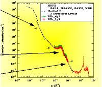
High Density Polyethylene showing XRD at high-q, SAXS at intermediate q and LS (light scattering) at low-q. Two Porod Regimes are observed.

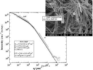
Light Scattering and SAXS from non-woven mat of micron scale fiber glass.

There are three other general categories of power-laws that are well defined in small-angle scattering, A) Surface-Fractal Laws, B) Diffuse interface Laws and C) Mass-Fractal or Dimensional Laws . Additionally there is the possiblity of D) polydispersity of particle size leading to power-law decays.

A) Surface Fractal Laws.

Systems that do not have smooth surfaces are often described by a scaling law where the surface area, S(r), is a function of the size of measurement. For example, the coastline of an island will increase if it is measured with smaller rulers since smaller rulers are capable of measuring the nooks and cranies of the coast line. For a smooth surface S(r) = r², and for a rough surface S(r) = r^ds, where d_s is the surface fractal dimension that varies from 2 to 3. Inserting such a scaling law into the discussion of Porod's Law above, yields I(q) proportional to q^ds-6. Surface fractals display power-law decays weaker than Porod's Law and are termed positive deviations from Porod's Law.

B) Diffuse interfaces.

C) Dimensional scattering laws.

Particles can be described in terms of their dimension in the sense that a rod is 1-D, a disk 2-D and a sphere 3-D. Such a dimensional description implies that the mass of the object depends on the size of observation, "r", raised to the dimension. Because of this it is natural to expect power-law scattering to result form such low dimension objects. Consider that scattering from a rod is observed at "r" = 1/q between the rod length, L, and the rod diameter, D. Then the number of scattering elements in the rod of size "r" is equal to L/r or Lq. The number of electrons per scattering element is given by rD² or D²/q. Using equation (1) we have I(q) = LD⁴/q, or a q^-1 decay in intensity for the 1-D object.

For a disk at size scales, r = 1/q, between the disk diameter, D, and thickness, t, the number of scattering domains is equal to the disk area, D², divided by the scattering domain size, r², or N_p = D²/r² = D²q². The number of electrons per scattering domain is given by the volume of a domain, r²t= t/q². Equation 1 yields I(q) = D²t²/q², or I(q) proportional to 1/q². Again the scattering is proportional to q^-df where d_f is the dimension of the object.

For a mass-fractal object such as a polymer coil the mass is given by the size raised to the dimension, i.e. for a polymer coil the end to end distance R is given by n^1/2 l, so the mass, n is proportional to R². In this sense a Gaussian polymer coil is a 2-D object. If such an object is broken into scattering elements of size r, the number of such elements is given by R²/r² = R²q² and the number of electrons in an element is n_e = r² = 1/q². Then equation 1 yields I(q) = R²/q², or I(q) is proportional to 1/q^df.

D) Polydisperse Particles

Many systems display dispersion in particle size in the small-angle regime. In some cases these dispersions are broad enough that they can be observed in terms of a power-law regime in scattering, i.e. when the dispersion in size occurs over a decade or more in size.

We have so far discussed power-law decays in scattering that are mostly defined between two size limits, i.e. for a rod a power-law decay of q^-1 is observed between the rod length and the rod diameter. Power-laws merge with a generic description of a discrete size at these limits, i.e. at q = 1/L or q = 1/D for a rod. For an isotropic system we can consider a particle in an average sense by allowing the particle structure to be averaged with respect to position and rotation.

The scattering event involves interference from waves emanating from two points in the particle separated by a distance r = 1/q. Then the probability of constructive interference involves the probability that given a point lying in an average particle, one finds a second point also in the average particle at a distance r = 1/q. For an isotropic system one must consider first averaging any starting point in a particle and secondly averaging any direction for the vector r. This leads to a double summation that is identical to the determination of the moment of inertia for a particle. When the electron density is used as the weighting rather than the mass density, this moment of inertia is called the radius of gyration of the particle. For a system of disperse shaped and sized particles the radius of gyration reflects a second moment of the distribution of the shape and size about the mean.

The process of obtaining R_g involves two steps, first averaging all possible positions in the particle from which a vector "r" can start and be within the particle. Second, determining the probability that a randomly directed vector "r" from an arbitrary starting point in the particle will fall in the particle. The meaning of this probability p(r), in the vicinity of r = the particle size, can be graphically represented by a Gaussian probability cloud created by the summation of all possible positions of the particle where the center of the probability cloud is in the particle phase.

At very low q this corresponds to the volume fraction particles squared. At sizes, r = 1/q, close to the average particle size or radius or gyration, this probability is reflected by a decaying exponential function. The decaying exponential function can be written in terms or r or in terms of q. (Fourier transform of a Gaussian distribution is a Gaussian distribution). Such an analysis leads to Guinier's Law, where the average size is reflected in the radius of gyration, Rg. Rg is the moment of inertia for the particle using the electron density rather than the mass as a weighting factor.

I(q) = N_p n_e² exp(-q²R_g²/3)

Sphere: radius R

I(q) = N n²{3(sinqR - qR cosqR)/(q³R³)}²

R_g = R/1.29 = RÃ(3/5)

Rod: Length 2H; Diameter 2R

R_{g overall} = R²/2 + H²/3

Disk: diameter 2R; thickness 2H

R_{g overall} = R²/2 + H²/3

Gaussian Polymer Coil: n persistence units; l persistence length

I(q) = I₀ {2(Q - 1+exp(-Q)}/Q²

Q = q²R_g²

R_{g overall} = n^1/2l/Ã6

I(q) = G exp(q²R_g²/3) + B q*^-P

q* = q/(erf(qR_g/Ã6))³

Small-Angle Scattering from Polymeric Mass Fractals of Arbitrary Mass-Fractal Dimension, Beaucage, G. , J. Appl. Crystallogr. (1996), 29, 134-146.

Approximations leading to a unified exponential/power-law approach to small-angle scattering, Beaucage, G., J. Appl. Crystallogr. (1995), 28(6), 717-28.