G. R. Strobl, Chapter 5 "The Physics of Polymers, 2'nd Ed." Springer, NY, (1997).
J. Ferry, "Viscoelastic Behavior of Polymers"
Chapter 3: Specific Relaxations
There are many types of relaxation processes that can occur in polymers. The identification of the details of these processes and how they relate to chemical structure is of primary interest in dynamic measurements. Generally, the specific relaxation processes are observed to display fairly discrete regions of activity in frequency. If several identifiable regimes are observed they are conventionally labeled by Greek letters starting from the highest temperature, lowest frequency or rate, 1/
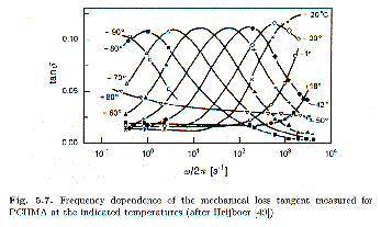
t. Typically, the glass transition is the a-absorption process, for example, reflecting relatively slow, long range motion observed at low frequency and relatively high temperature. Higher frequency transitions might involve side-group motions or conformational changes in side groups. These transitions, b and g are usually observed in the glassy state and correspond to low-temperature transitions. In some materials new transitions occur when polymers are confined to crystalline structures or when chains absorb to filler material for instance.Figure 5.7 from Strobl p. 214 shows the behavior of a simple activated
g-transition in an acrylic polymer with a cyclohexane side-group in terms of the loss tangent, tan d (w)= G"(w)/G’(w). The side-group can display a conformational transition between a chair and a boat ring conformation. This g-transition process is thermally activated, does not depend on the molecluar weight of the polymer and is seen for different main chain polymers that possess this cyclohexane side-group. For these reasons it is a nice candidate to demonstrate the behavior of a polymeric transition. The —60°C curve in figure 5.7 displays the symmetry (on the log w axis) characteristic of a Debye-Process discussed in chapter 2. The width at half-height is about 2 decades in frequency (greater than the 1.2 limit for relaxation processes.
The dependence of the frequency of maximum relaxation on temperature indicates that the process may be thermally activated. A simple, thermally activated process will follow an Arrhenius behavior,
![]()
where Ea is the activation energy, or energy barrier, for the transition from chair to boat conformation for the cyclohexane group. K is the relaxation time for T => °, i.e. the relaxation time in the absence of energy barriers,
t0. The relaxation time can be obtained from the frequency of the maximum in the curves in figure 5, t = 1/wmax. Taking the log of the above equation for the Arrhenius relaxation time we have, log(t) = log(K) + (Ea/k) (1/T). So a log-linear plot of t (or w) versus 1/T should yield a line whose intercept is log(K) and whose slope is (Ea/k). Such a plot is shown in Strobl’s figure 5.8, from which Ea = 47 kJ/mole.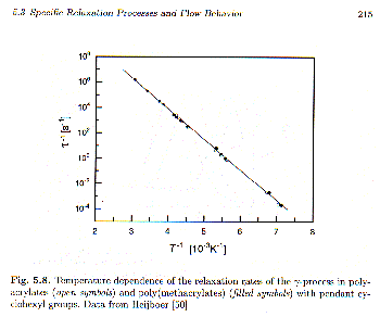
Figure 5.9 (Strobl) shows the temperature dependence of tan
d for different frequencies. Because of the Arrhenius relationship, given above, there is a strong correspondence between the frequency and the temperature plots. This correspondence between time (frequency) and temperature is known as time-temperature superposition and is a basic characteristic of thermally activated relaxation (Debye-type) processes. Dynamic properties of Debye-processes depend on wt as a free parameter. If the process is thermally activated such as in an Arrhenius form, then there is a direct relationship between relaxation time or measurement frequency and temperature through an exponential function. For the complex compliance, J*(log wt), we have, log wt = log w + logt0 + Ea log e/kT. Equivalent changes in J*(log wt) can then be achieved by variation in frequency, w, or variation in temperature, T.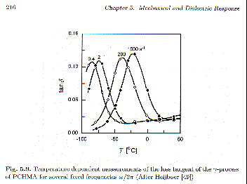
Time-temperature superposition indicates that the curves in figure 5.8 or figure 5.9 have the same values at corresponding positions, i.e. at the peak position tan
d should have the same value. This is roughly followed for the tan d curves of this g-transition. The curves in figure 5.8 or 5.9, then can be shifted along the corresponding x-axis by a shift-factor, aT or aw, so that the curves from different conditions overlap. This was done by Strobl in figure 5.10 for G’ and G".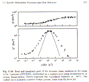
Figure 5.10 also shows a comparison with a simple, single-relaxation time Debye-Process (lower plot). The measured relaxation shows some broadening indicating a more complex system than a simple Debye-process. Only broadening of such a peak is possible for a relaxation process, i.e. the peak can not be narrower than the Debye-process if it corresponds to a relaxation phenomena.
Calculation of the shift-factor, aT, for the construction of a master-curve such as that shown in figure 5.10 will be discussed after we consider the characteristic features of polymer systems near the glass transition temperature.
Characteristic Features of Polymer Creep Compliance, Tensile and Shear Modulus Near Tg:
Strobl’s figure 5.12 shows the characteristic features of compliance, J’, for a polymer as a function of time = 1/
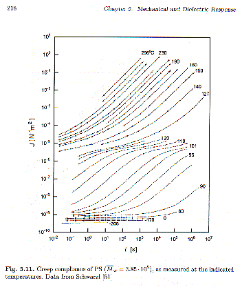
w. Such a curve might be constructed from a series of dynamic mechanical scans after shifting of the curves to form a master curve, figure 5.11. The compliance typically varies over 109 orders in compliance and over 20 orders in time! The creep compliance is very small (10-9 m2/N) and constant at short times (high frequency) reflecting the glassy state. This is followed in time by the a-process at the glass-transition where the features of a Debye-like relaxation process are shown. For relatively high-molecular weights a molecular weight dependent plateau region is observed (10-5 m2/N) associated with an entanglement network that does not have time to relax. At longest times linear behavior is seen indicating viscous flow, dJ’/dt =dg12(t)/dt (1/s12) = 1/h.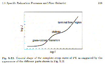
The composite curves shown in Strobl’s figure 5.11, below,
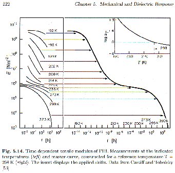
Strobl’s figure 5.14 shows a similar plot for the tensile modulus of polyisobutylene. The same regimes discussed for the creep compliance curve, above, exist in this curve.
Simple Empirical Models for Polymer Transitions:
Polymer transitions involve more than one relaxation time as indicated by the comparison with a simple, Debye-process in figure 5.10. This is also true for the
a-transition or glass-transition. The time dependent modulus, E(t), in a stress relaxation measurement follows E(t) = Er +DE exp(-t/t) for a single relaxation time Debye-process. One way to empirically broaden this transition behavior is to arbitrarily raise the time ratio in the exponential to a power, b, less than 1,![]()
where this Williams-Watt Function depends on two parameters, a time scale,
t, and the power, b. This kind of function is called a stretched-exponential for obvious reasons. For the glass transition temperature b is typically 0.5 (Strobl p. 222). The Williams-Watt Function describes the "knee" part of the modulus curve shown in figure 5.14 of Strobl (short time or high frequency). The log-log plot of figure 5.14 shows a linear region following this knee that can not be described by an exponential decay. This power-law regime is empirically described by the function E(t) = K t-n. Typically it is observed that n = 1/2.Following the glass transition exponential and power law regimes in time is the plateau regime for uncrosslinked polymers. This plateau is related to an entanglement network and is only observed for polymers above the entanglement molecular weight. Figure 5.15 of Strobl shows that this plateau regime grows in extent with molecular weight.
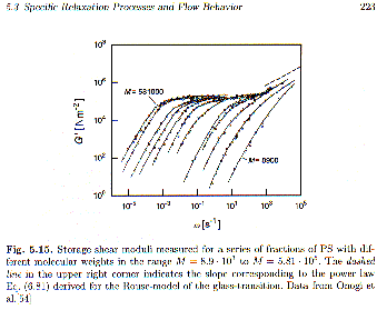
Following the plateau regime a second power law regime is observed in the log-log plot of figure 5.15. The slope in this regime is 2 for a frequency plot and —2 for a time plot, G’(
w) = K’ h w2 or E(t) = K h t-2.