 (1)
(1)Small-Angle X-ray (Neutron) Scattering (SAXS)
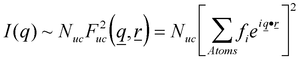
We have considered that the intensity of a scattered or diffracted beam from a crystal is proportional to the number of unit cells Nuc times the square of the structure factor for a unit cell, Fuc,
(1)
where q is related to the scattering angle, 2q (or sometimes q), by q = 4psin(q)/l, r is a real space vector that describes the position of an atom, f is the atomic form factor that describes the effective number of electrons associated with an atom including interference associated with electrons within an atom. The dot product of q and r yields a phase angle, fi. In XRD q is given by 2p times the reciprocal space location of the reflecting plane (h,k,l) and r is given by the real space location of the atom [u,v,w]. These definitions of the scattering vector and the real space vector yield the von Laue equations for diffraction (Bragg's law in 3-d space).
At large size scales, 1 nm to 1 mm (the nano- to colloidal scales), matter is not as well organized as matter at atomic size scales. There are several reasons for this:
1) Atoms of the same type are identical in size and shape while materials at nano- to colloidal scales are never perfect. Imperfect unit cells can not pack perfectly just as you can not make a perfect repeat pattern from natural rocks while bricks can be stacked in a perfect pattern.
2) Atoms fully follow thermodynamics since they occur in great numbers and materials are composed of collections of such huge numbers of small particles that equilibrate thermally, through motion in space. On the nano- to colloidal scales thermodynamics breaks down at some point (probably depending on temperature) due to the relatively large mass of structures on these size scales. Thermodynamic interactions are the basis of crystallization, for instance the crystalline melting point is the ratio of the enthalpy difference by the entropy difference between the melt and the crystalline state. For colloidal to nano-scale materials entropy is not well defined due to small number density and relatively large mass.
3) The relatively low number density of matter at colloidal to nano-scales compared to atomic scales means that systems tend more often to be effectively dilute (gas like) while the large number density, due to size, of atomic scale structures makes it difficult, or impossible in some cases, to achieve a gas like dilution. The effective number density is also reduced by the smaller thermal mean free path of material at the nano- to colloidal scales, that is material at these size scales probe a much smaller volume relative to their size when compared to atoms at thermal equilibrium. This means that the probability of contact between objects (what is the salient part of the number concentration) is much lower.
4) Objects at the nano- to colloidal scales tend to display a higher polydispersity in asymmetry and size relative to atoms. These factors hinder formation of repeating patterns in space.
Other structural features that are fairly unique to the nano to colloidal scales include:
1) The tendency towards asymmetry of structure, platelets or rod like particles. Asymmetry enhances ordering in the nano- to colloidal regime and there are many cases of Bragg-like scattering in this regime of size due to asymmetry. This differs from atomic scale structures where large aspect ratios are uncommon. (Liquid crystalline polymers, block copolymers and lamellar polymer crystals are some examples.)
2) Static electric charge is also a major factor leading to enhancement of order on the colloidal to nano-scales. Colloidal silica and soap micelles are examples of order on the nano- to colloidal scales.
Both of these issues are important to the study of biological materials, especially in aqueous environments on nano- to colloidal scales.
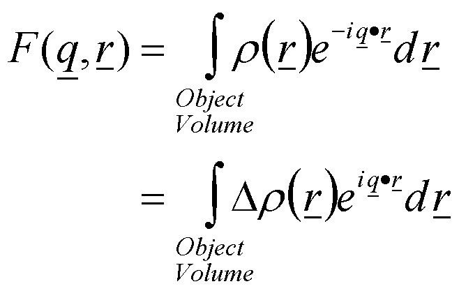
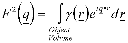
Because of the effective dilution at large size scales and the lack of regular order eq. (1) is not useful for interpretation of small-angle scattering. A more general form of eq. (1) is needed based on what we have learned from diffraction. In small-angle scattering we are generally interested in the structure of objects rather than their arrangement in space in a lattice. For example, rod like virus proteins (tobacco mosaic virus) can scatter in the small angle regime (1 Å-1 > q > 0.0001 Å-1). It might be desirable to understand the relationship between the aspect ratio of these rod-like particles (A = L/D) as a function of their thermal degeneration. This is quite a different problem from understanding the crystalline transitions of nylon at high pressures for instance. In order to understand the structure of a single, isolated (effectively dilute) particle we must have a model for the distribution of electrons in the structure (fi in eq. 1). From XRD we understand that for many atomic crystals, such as NaCl, fi is described by the phase relationship between multiple atoms at a lattice site in exactly the same manner as the description of the location of multiple lattice sites in a unit cell (crystalline structure factor F in eq. (1)). However, complex and large objects in the nano- to colloidal regime do not display a simple arrangement of electrons. Generally, the number of electrons per volume, or electron density r(r), is a continuously varying function of position within the object. The electron density is not a stepwise function as it is in a unit cell, that is there are no specific positions of electron centers, lattice sites, in a large complex object when viewed at nano- to colloidal scales. For these reasons the structure factor, F, in eq. (1) must be modified so that it includes an integral over the volume of the isolated particle and so that it includes a continuous description of the electron density distribution in the object,
 (2)
(2)
The electron density r(r) can be decomposed into the mean value <r(r,t)> for the dilute collection of particles and the contribution due to deviations from this mean value, Dr(r,t), which can have positive or negative values. r(r) = <r(r)> + Dr(r). t is time and it is included to emphasize that the fluctuations, Dr(r,t), can be due to spatial distribution or due to thermal motion of the nano- to colloidal scale particles. Here we will only consider a spatial distribution. Then eq. (2) leads to two integrals, the first of which displays a constant exponential prefactor, <r(r)>, so that the integral over volume (of all irradiated space) is 0 since there is a uniform distribution of average electron density in space. The second equality in eq. (2) reflects the dependence of the structure factor on fluctuations in electron density (in space or time). (The association with fluctuations indicates that there may be a link between small-angle scattering and thermodynamics since fluctuation of density due to thermal motion is the basis of the isothermal compressability of a homogeneous material.)
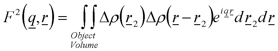
Since Dr(r) is an unknown continuous function that may be complicated in form, eq. (2) can not be easily reduced to a more manageable form, especially as a general rule. Further, eq. (2) is generally a complex number with positive and negative values. Equation (2) does not yield direct access to a statistical description of the object which is inherent in the small-angle scattering measurement. The complex, phase information present in eq. (2) can be removed by considering the scattered intensity which is proportional to the square of eq. (2) as previously discussed for diffraction, especially for the structure factor of hexagonal lattices where a complicated complex function results for the unit cell structure factor. For eq. (2) F2, links directly to a statistical description of the object native to computer simulations of structure and theory, the pairwise correlation function, g(r), making small-angle scattering an important tool for judging the results of structural simulations and theoretical analysis of materials.
Consider two points in the object of eq. (2) separated by a vector r, r1 and r2, so r = r2-r1. r2 is then given by r1 + r, and,
 (3)
(3)
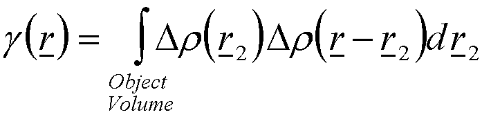
Equation (3) contains two integrals, one involving r and the other r2. The complex part of eq. (3) involves only r so this term can be treated as a constant in the integral over r2. We need to consider the integral over r2 independently since it represents one of the most important functions in our understanding of the structure of materials, the pairwise correlation function, g(r), which is a statistical description of the average structure in real space,
 (4)
(4)
The correlation function can be understood from a line throwing experiment. For lines of length r, g(r) is proportional to the probability that if one end of a line is in the object volume, that another randomly placed end of the line will also fall in the object. The correlation function is 0 for lines larger than the objects largest length and is Dr2 when r = 0. Between these limits the correlation function decays with a functionality that reflects the objects structure in a somewhat complex way. The correlation function is useful in describing objects of complex structure, for example, to compare different types of trees analytically one could calculate the correlation function and arrive at a number that was unique to evergreen trees. Such an analytic descriptor of trees is not possible in a normal non-integral approach to structure. The correlation function can yield average properties of the object through integrals and other manipulations such as the surface area, the average volume and mean object size. If rather than considering multiple origins for the line of length r in a fixed object, we consider a fixed line and move the object to all possible locations in 3-d space where the first end of the line lies in the particle and average the structure of the object in these positions we arrive a different understanding of the correlation function. For such a spatially averaged object differences in structure are blurred to a decay curve. The correlation function represents the square of electron density for such an averaged object. Equation (3) using eq. (4) becomes,
 (5)
(5)
In a small-angle scattering experiment many such objects are simultaneously measured and the average <F2> is observed,
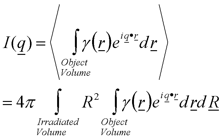 (6)
(6)
Equation (6) shows that the scattered intensity is a Fourier transform of the pairwise distribution function.
It should be clear that an object described by the correlation function is symmetric about a center of mass, R0. Further, spatial averaging over all such objects in the irradiated volume further ensures symmetry of the average structural probability described by the correlation function. For such symmetry about the center of mass we can ignore the vector nature of r and q, and simplify equation (6) following Debye (as described in Guinier and Fournet 1955 for instance),
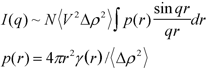 (7)
(7)
where p(r) is the normalized total pairwise distribution function. p(r) has a value of 0 at r = 0 (since r2 is 0 and g(r) is finite) and also has a value of 0 for r larger than the largest object size since g(r) goes to 0 at large r. p(r) shows a peak in r near a mean object size. The integral of p(r) over all r is 1. p(r) includes the increase in area associated with larger r so it is a total probability rather than a linear density based probability. Equation (7) is sometimes called the Debye scattering function since it was derived by Debye.
Equation (7) shows that the scattered intensity is proportional to the number density of objects in the scattering volume, N, and is proportional to the volume of the scattering elements, V. The integral term describes the interference effects associated with the distribution of electrons in an average object.
Equation (7) indicates a dimensionless length, R = qr. We can make the substitution r = R/q. The integral in eq. (7) is 1 when R/q >> D, or at small q compared to R/D, where D is the diameter of the object under consideration. This condition is possible for any size D if a small enough q value is used at least in approximation. Alternatively, a large object could be subdivided using the structural scaling features of an object to sizes that meet this restriction as described below.
If we consider a collection of objects of size r that compose a larger object such that the component objects meet the restriction that R/q >> D, an approximation of equation 7 can be made,
![]() (8)
(8)
Using eq. (8) many of the the basic equations of small-angle scattering can be obtained (in approximation). Additionally, it is possible to understand general features of the small-angle scattering curve such as the tendency to display power-law scattering and the general decay of the scattered intensity in q.
General Decay of I(q) in q:
For any object divided into m smaller objects so that D becomes smaller and q/R becomes larger, we have that Nm = m N0, where N0 is the original number of objects and Nm is the number of component objects. The size of the component objects is smaller than the size of the original object and the size, r follows, rm ~ r0/m1/df. The volume scales with Vm ~ V0/m3/df, where df is the dimension of the object which varies from 1 to 3. Then I(q), from equation (8), must decay with m and with q/R. We have ignored interference between component parts of the original object which would enhance the decay in I(q). (For instance, in a 3d object the scattering from all internal structure is subject to destructive interference since there is always a component of scattering out of phase by half of the wavelength.) The general tendency of intensity to decay in angle or in q in the small angle regime is related to the relationship between I, N and V2.
Porod's Law:
When two phases meet at a smooth sharp interface with phases of infinite extent the constant contrast factor within each of the two phases is constant leading to total destructive interference between waves from different parts of the phase. For phases that are much larger than the size of observation, r = R/q, the source of scattering is the interface. The interface can be decomposed into a series of spheres of size r as shown in Fig. 1. N(r) = A/r2 where A is the surface area of
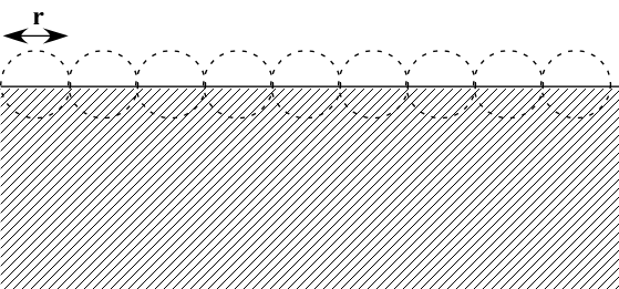
Figure 1. Schematic of smooth sharp surface between infinite extent phases.
the interface. The volume of a domain scales with r3 so,
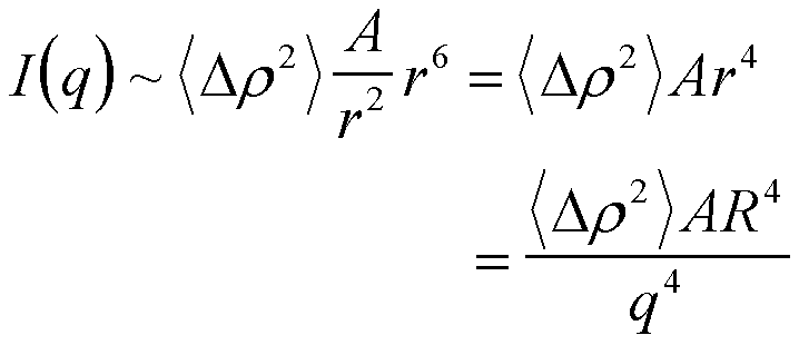 (9)
(9)
Equation (9) is used to determine the surface to volume ratio of materials on the nano- to colloidal scale using scattering.
Dimensional Scattering Laws:
An object such as a rod or a plate differs from a 3d object such as a cube or sphere in that the objects dimension, df, is not 3. Generally, an objects dimension must be equal to or less than the space in which it is embedded (generally 3) and larger than or equal to 1 (a rod). For objects of dimension 3 internal scattering does not exist due to total destructive interference between the component parts (Porod surface scattering). For low dimension objects, the internal interference associated with component objects not in a connected path is ignored following Debye (Debye scattering function for an ideal polymer coil, 1949). (For a 3d object we can not distinguish between connected and non-connected paths so this assumption fails for 3d objects.) For a rod, the assumption is totally correct since there are no component objects not along the connected path which is linear. Low dimension objects display at least two length scales, the overall size and the substructural size. For a rod these correspond with the length and the diameter. For a platelet the diameter and the thickness. Between these two size scales the object displays low dimensional scaling of mass (N) with size (V) so that a scaling relationship between I and q can be obtained using eq. (8).
For a rod the number of component elements of size r, N(r), when r is between L and D is L/r. The volume of a component element scales with rD2. Then the scattered intensity shows a power-law scaling of I(q) ~ LD4r = LD4R/q. For a disk with r between D and t, N(r) ~ D2/r2 and V ~r2t so I(q) ~ D2t2r2 = D2t2R2/q2. From these two examples we can see that the scattered intensity scales with I(q) ~ q-df, where df is the dimension of the object. This scaling law ignores non-connected interference between structural components. It is expected that this assumption will fail for df approaching 3.
The result for a rod and disk can be generalized for any object displaying ramified and convoluted structure. In general we can say that the mass of the object, N(r), will scale with the dimensionless size of the structure to the df power, (L/r)df, where L is the total structural size. The volume of a substructural element of size r scales with V(r) ~ rdfl(3-df), where l is the small dimensional size of the object such as the size of a primary particle, thickness or diameter. Equation (8) yields, I(q) ~ (L/r)df r2df l2(3-df) ~ Ldf l2(3-df) rdf ~ Ldf l2(3-df) Rdf /qdf.
Guinier Scattering:
The Porod surface scattering law and the dimensional scattering law indicate that we can expect power-law scaling of I(q) versus (q) for a variety of structures between size or q limits in the small-angle regime. It is natural to plot log(I(q)) versus log(q) to observe these regimes as lines. The power-law nature of scattering also indicates that we might expect a transition regime between power-law regimes. These transition regimes are observed when the r = R/q reaches the limiting size of a structure such as the overall size of an object. The object is considered in the context of the correlation function so that it is observed as a symmetrically decaying probability function that peaks at the center of mass of the object, R0. The scattered intensity is a Fourier transform of this function according to eq. (5). Then we should consider what form a pairwise distribution function for such an averaged object should take. It should not be surprising that we can generally describe such an object using a Gaussian Function which describes a random arrangement of matter centered on a mean value. The advantage of a Gaussian function is that the Fourier transform is well described by another Gaussian function, in this case,
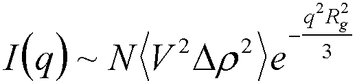 (10)
(10)
where Rg2 is the moment of inertia of the object or the square of the objects radius of gyration,
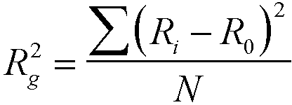 (11)
(11)
Equation (10) in a log-log plot is seen as a rapidly decaying knee.
Limits of Power-Law and Guinier Regimes and the Unified Equation:
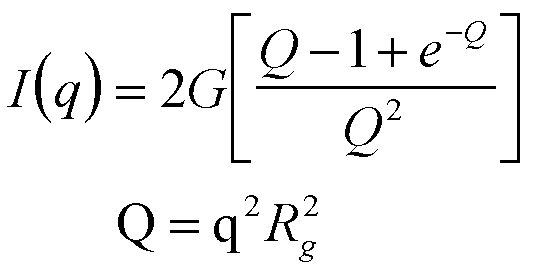
Most scattering at small angles from disordered materials can be described by a series power-law decays, I(q) = B q-P, separated by Guinier regimes, I(q) = G exp(-q2Rg2/3). The Guinier and power law regimes generally overlap to some extent making it necessary to consider a functional form that can describe both surface and mass scaling regimes (Porod and mass fractal laws) as well as the Guinier regime. Such functions exist for specific structures by calculation of the correlation function and through Fourier transformation of this function. For example the scattering function for monodisperse spheres of radius R is given by,
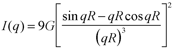 (12)
(12)
where G ~ N<Dr2V2>. Eq. (12) yields Porod's law at high-qR and Guinier's law at low-qR relative to qR = 1. Then eq. (12) describes the overlap between Guinier and Porod regimes for the specific structure of monodisperse spheres.
Similarly, the scattering function obtained by Debye for a Gaussian polymer chain describes the Guinier regime for the coil and the mass-fractal scaling regime, df = 2,
 (13)
(13)
For objects that are asymmetric such as rods and disks the functional form for I(q) must include an integral over the object's orientation so a direct functional form not involving an integral is not possible through a Fourier transform of the correlation function.
A generic scattering law that describes the overlap between Guinier and power-law regimes has been developed, the Unified function,
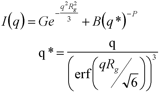 (14)
(14)
The Unified function can be extended to describe multiple power-law regimes (levels of structure),
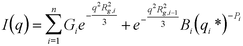 (15)
(15)
where n levels of structure are considered and where Rg, 0 = 0. Lower values of i correspond to smaller structures or higher-q so the numbering of structural levels begins at the smallest size. Equation (15) can reproduce the scaling features of all conventional scattering laws that do not involve correlations. It can be used for fractal scattering with non-integral scaling and can reproduce scattering curves from a variety of systems that have no analytic form such as scattering from rough surfaced particles.
Correlations:
As the concentration increases eqs. (8)-(15) must be modified to account for correlations between objects. For relatively low concentrations the interference between particles due to density can be approximated by multiplying eq. (8) ,for instance, by f (1-f) as described by Guinier and Fournet 1955, where f is the volume fraction of objects or particles. This modification should not be included if the particle correlations are dealt with directly through a functional modification of the scattering equation. For example, for mass fractal aggregates the mass fractal scaling regime accounts for the majority of primary particle correlations. Further, if correlations lead to a peak in the scattering data then the f(1-f) modification is not sufficient or appropriate. For spherically symmetric or disordered particles with no preferred or regular asymmetry the Born-Green approximation can account for correlations under the assumption that correlations can be described by a spherically symmetric correlation about the center of mass of a particle (Guinier and Fournet 1955). Under this approach the scattering from a structural level is modified by the function 1/(1+pA(q,x)) where A is the sphere amplitude function (square root of eq. (12) with G = 1) which depends on the average correlation distance, x (substituting for R in eq. (12)) and p is a factor that accounts for the order of packing or packing density. When p is 0 the system is dilute. For closest packing p is 5.82 as described by Guinier. For systems that display asymmetric objects such as stacked lamellae or rods the Born-Green approach will not work in its unmodified form. Often, such systems are dealt with by Fourier transforming the intensity to obtain the correlation function and analyzing the correlation function in terms of structural models. Alternatively, the Lorentzian corrected data, Iq2, can be analyzed for a Bragg spacing. These approaches are described by R.J. Roe (2000).
Small-Angle Neutron Scattering:
The basic scattering laws described for x-rays are essentially identical when used in a neutron scattering experiment except that the electron density is replaced by the neutron cross section. The neutron cross section does not depend on the atomic number and is basically random about the periodic table. Hydrogen and deuterium which have indistinguishable chemical properties and x-ray contrast have the most widely spaced neutron cross sections allowing for deuterium tagging especially of hydrocarbons for contrast enhancement. The neutron scattering experiment is done at a national user facility such as NIST in Washington, Argonne National Laboratory in Chicago, Oak Ridge National Laboratory in Tennessee, or Los Alamos National Laboratory in New Mexico. (The facility at Brookhaven National Laboratory in New York has been recently closed.) Facilities for Neutron Scattering also exist in France, Britain, Germany, Switzerland, Japan and a number of other countries. In addition to the contrast enhancements possible with neutrons, the absorption coefficient is much lower for high atomic number materials such as metals allowing for measurement on much thicker samples, up to several inches for steel for instance, allowing for measurement on industrial samples and on samples that could not be examined using x-rays. The neutron measurement is typically an order of magnitude larger in size so that a 1 cm beam is common with a 10 meter flight path for a pinhole camera. Beam time at a neutron scattering facility is usually obtained either by a short proposal or by contacting the instrument scientist. Facilities are provided free of charge for publishable research and with a small fee for proprietary work. Generally, the fee for neutron scattering is a small fraction of the costs associated with an in house SAXS facility.