Isothermal Viscoelastic Fiber Spinning Model
![]()
images: www.ipfdd.de/research/res25/model/FiberModeling1.html and http://www.ipfdd.de/research/res53/res53.html
Fiber spinning is a polymer process that involves extruding a polymer through a capillary die and uniaxially drawing the extrudate into a thin fiber. This process is commercially used to produce fibers for carpeting and clothing, as well as fiber optic cables. A similar process is also used for non-polymeric systems, such as glass filament.
The following figure shows a fiber spinning system:
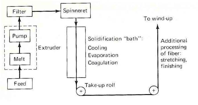
image: Middleman, S., Fundamentals of Polymer Processing, 1st edition, McGraw-Hill, 1977.
The polymer is fed into an extruder, where it is heated, sheared, and pumped through a filtering system to eliminate any gels or unmelts that may be present in the extrudate. The polymer then passes through a die called a spinneret that has several small, annular dies. The extrudate exits the die in a molten strand of polymer that is several times larger than the desired final gauge. The molten extrudate is then uniaxially drawn in the machine direction to the desired gauge. During this drawing process, the molten polymer solidifies, typically by a quenched water bath or simply by cooling in ambient air. The fiber is then wound on a spool and is used in a secondary commercial process to produce goods.
The portion of the process where we are particularly interested in is the section between the exit of the die and the take up roll. From a polymer scientist’s perspective, this is the section of greatest intrigue…with various dynamic processes occurring simultaneously, including crystallization and orientation.
Melt Spun Fiber Stretching
From our description of the fiber spinning process, we see that the cross sectional area of the fiber and the radius vary with position along the z-axis, with z representing the drawing direction. Ideally, the goal is to simultaneously solve the r and z components of the equation of motion and the thermal energy balance, the continuity equation and the appropriate boundary conditions. Doing so has proven complicated, given the non-linear viscoelastic nature of polymers. Kase and Matsuo were the first to consider non-isothermal fiber drawing with Han giving the following generalized approach to their model.
Assuming steady state, the only velocity component is vz(z), meaning T=T(z). This means the momentum balance equation is:

And the thermal energy balance equation is:

Where e is the emissivity, G is the mass flow rate and is given by:
![]()
And FD is the air drag force per unit area and is given by:

r is the density and m is the viscosity. The subscript “a” refers to ambient conditions.
And h is the heat transfer coefficient and is given by:

Where K is an adjustable parameter and k is the thermal conductivity.
Han combined the momentum and thermal balance transport equations and included a power law in tension constitutive equation with a temperature dependent viscosity term to yield:

Where B is a parameter for the pressure dependence on viscosity and a is calculated by:
![]()
These equations are then solved numerically and is a reasonable representation until the point where crystallization begins and the rate of cooling slows down. Other issues associated with the fiber drawing process that are not addressed with this particular model are radial temperature gradients (addressed by Morrison) and flow (stress) induced crystallization (addressed by Spruiell and White).
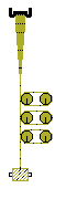
Structural effects (i.e. the way the crystallites form, are arranged, and are structured) are also of importance in understanding the properties of drawn polymers and can vary greatly with operating conditions. Dees and Spruiell studied such effects in HDPE. The following figure represents the morphology of the polymer crystallites as a result of varying take up speeds (or uz).
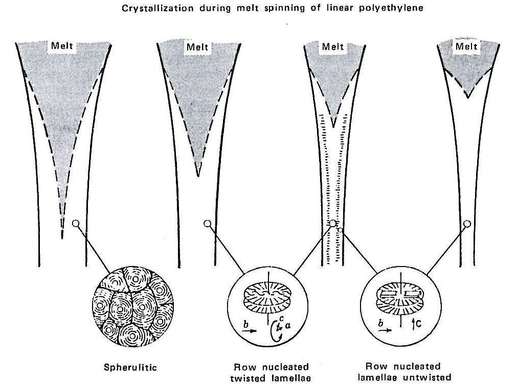
image: Tadmor, Z., Gogos, C. G., Principles of Polymer Processing, 1st edition, Wiley, 1979.
At low line speeds (or take up velocities), spherulitic structures are formed. As the rate increases, lamellae are formed. At moderate velocities, twisted lamellae are present and as the rate increases, the untwisted form initially described by Keller and Machin are evident.
The final section in this
description of the fiber spinning process will cover draw resonance and
spinnability. Draw resonances results in a regular and sustained periodic
variation in the fiber’s diameter. Spinnability is the ability to draw a fiber
without it breaking. This is also commonly referred to as “melt strength”. This
phenomenon is the result of instability of mass flow between the die and the
take up roll, also known as the draw gap. The rate of mass entering the gap
remains constant, but the rate leaving is not since only the take up speed is
regulated and the diameter of the fiber is not. So, if the fiber becomes
instantaneously thinner at the take up roll, the portion of the fiber above the
thin spot becomes proportionally thicker. Eventually, this thick spot reaches
the take up roll, and by conservation of mass, the fiber above the take up roll
becomes thinner. Observations by Miller and Kase report that if solidification
takes place prior to the take up roll, no resonance is observed. White and Ide
observed that increasing the residence time of the process increases the
resonance period seen in the fiber. For isothermal drawing, the presence of
draw resonance is independent of line speed and dependent on draw ratio. For
Newtonian fluids, draw resonance occurs at a draw ratio of 20.2 (per Pearson and
Shah). For viscoelastic polymer melts of polyolefins (HDPE, LDPE, PP) and PS, a
critical draw ratio can be as low as 3 (per Cruz-Saenz, Donnelly, and
Weinberger).
The critical draw ratio depends on the power law index (n) and the viscoelastic dimensionless number (N) calculated by the following:

Where m is the consistency index from the power law model, L is the drawing gap, G is the tensile modulus, and V0 is the spinnerette velocity. Refer to the rheology web page of this site for a review of the rheological terms.
The following figure is commonly used to study the stability of the fiber drawing process and is a plot of draw ratio versus N.
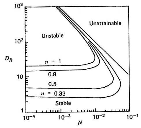
image: Tadmor, Z., Gogos, C. G., Principles of Polymer Processing, 1st edition, Wiley, 1979.
We see in the figure that at high draw ratios we have an unstable region at low values of N, a narrow operating range of N where polymers of various n values converge, and an unattainable (i.e. the fiber breaks) region at high values of N. Stable drawing is achievable at low draw ration, with stability improving at higher draw ratios with higher values of n. Experimentally, we know that increasing the drawing temperature, higher draw ratios are attainable without draw resonance. Upon reviewing the equation for N, this makes sense. Increasing the temperature decreases G and increases m, which increases N and results in higher draw ratios.
For a more detailed mathematical model of the fiber spinning process, the reader is referred to Middleman’s Chapter 9.