Figure 1.
Homogeneous Nucleation
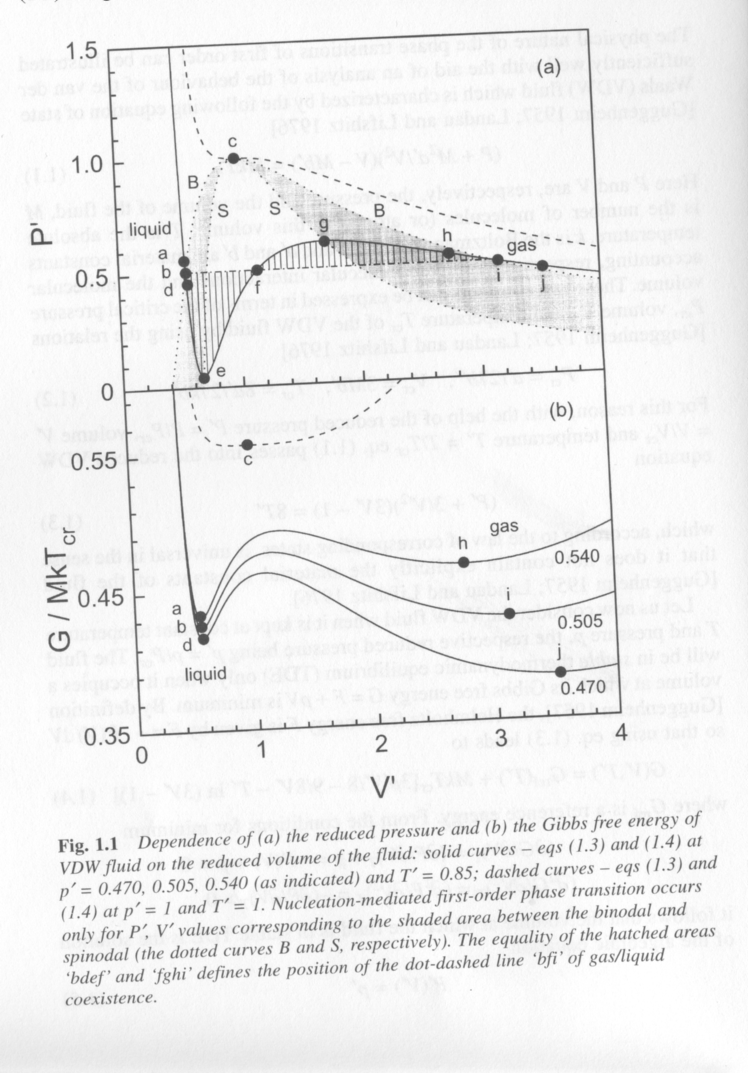
For a van der Waals fluid (non-ideal gas/liquid with van der Waals ineractions) condensation of the liquid phase or evaporation of the liquid is governed by the equation of state. For a fixed number density of atoms, changes in volume, pressure or temperature can drive the gas or liquid into an unstable state. Figure 1 from Kashchiev shows a plot of reduced pressure, P/Pcr, versus reduced volume, V/Vcr, where cr indicates the critical point for the system (point c) and a plot of Gibbs free energy versus the same V/Vcr x-axis. The temperature is below the critical point, Tcr so two phases, gas and liquid can be in coexistence as indicated by the words liquid, at low volume, and gas, at high volume in the two plots. We can consider what constitutes equilibrium in this system, what is the composition of phases at equilibrium, when can the system undergo a first order transition to lead to new phases.
Figure 1.
The solid curves in Fig. 1 correspond to the equation of state for the Van der Waals fluid (top) and and expression for the free energy obtained from derivatives of the equaiton of state. The three solid curves in the bottom plot are for three reduced pressures which are indicated at the right. The dashed curve is at the critical temperature in the top plot and at the critical pressure and temperature in the bottom plot.
The bottom plot is probably most familiar to students of materials science and physical chemistry. Minima in this curve (first derivative 0) represent approximately the binodal points for the composition of phase equilibria, inflections (second derivative 0) correspond approximately to the spinodal (limits of spontaneous decomposition) and the maxima (third derivative 0) is approximately the critical point. Phase separation occurs between the binodal points but a region of metastability exists between the binodal and spinodal points where phase separation will only proceed if a nucleus exists. Then we can define two types of nucleation, homogeneous nucleation between the spinodals and heterogeneous nucleation (nucleation on a preexisting nucleus or seed).
From the free energy plot it is possible to sketch in the binodal and spinodal points on the P' versus V' plot (top). This is shown with the dot-dash lines in Fig. 1 at the top. The hatched areas represent the meta-stable regions. The central white region of the plot is the region where spontaneous, homogeneous nucleation will occur since composition fluctuations are unstable for any size of a spontaneous fluctuation in this region. Above the critical point a supercritical state is formed which is not a liquid or a gas but something similar to a liquid but with no surface tension, that is without a real surface.
For a gas at a fixed pressure, reducing the volume will lead to a state first of meta-stability (hatched area) then to a state of instability where spontaneous separation into a liquid and gas phase at equilibrium will occur. This would be a horizontal track across the top plot at P' ~ 0.54. Depending on the "quench-depth" that is the difference between the spinodal line and the V' of the system, two phases will coexist in equilibrium; liquid phase a and gas phase h.
The P' curve in Fig. 1 is calculated directly from the equation of state and ignores thermodynamic stability. As the equation of state liquid (low V') is expanded the pressure P' predicted by the equation of state drops rapidly. Being a non-ideal liquid it displays a small degree of compressibility. This reduction in pressure with volume is predicted until the spinodal point where the fluid pressure increases rapidly with increasing V'. At the second spinodal point, g, normal reduction in pressure with increase in volume is predicted. In the meta-stable region, shaded area, the pressure decreases with volume but at a moderated rate compared to the stable liquid or stable gas. The equilibrium pressure for the quenched fluid is decided by a horizontal line where the two hatched areas are equal. This is called a Maxwell rule.
Phase equilibria, thermodynamic equilibrium between two phases, is defined by equality of chemical potential, mi = dG/dni, between two phases, where i is one of the two phases. The chemical potential can be approximated by the slope of the free energy versus volume curve in fig. 1. Fig. 2 shows a plot of chemical potential for a Van der Waals fluid versus reduced pressure, P', at T' = 0.85, solid curve and at the critical temperature T' = 1. At low pressure a gas exists, Fig. 1. The gas passes through the binodal, b, spinodal, e, and spinodal g, and finally the binodal, i, to the liquid state in Fig. 2. Within the spinodal region (between e and g) the chemical potential drops to the binodal value (b, i) through homogeneous nucleation of a new phase. The lower plot in Fig. 2 shows the discontinuity in the first derivative of chemical potential for this first order transition. The equilibrium pressure is defined by the binodal point (b,i) in Figs. 1 and 2. The system is supersaturated in either the liquid or gas phase when it is between the spinodal points (e and g). The driving force for phase separation is the difference in chemical potential between the supersaturated gas or liquid and the equilibrium chemical potential defined by the spinodal.
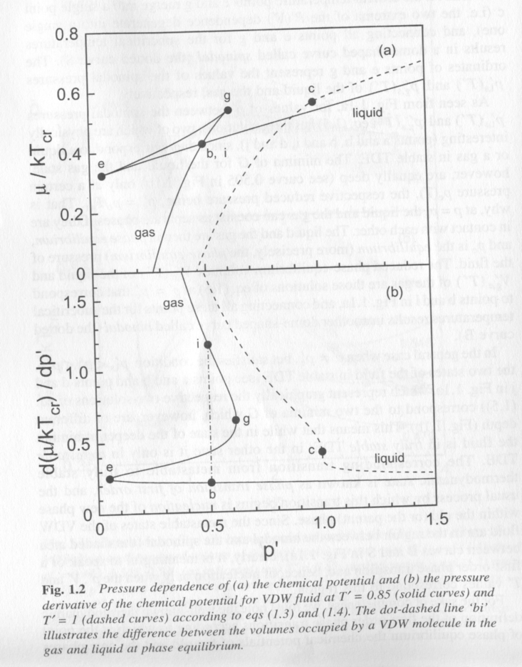
Figure 2.
Supersaturation:
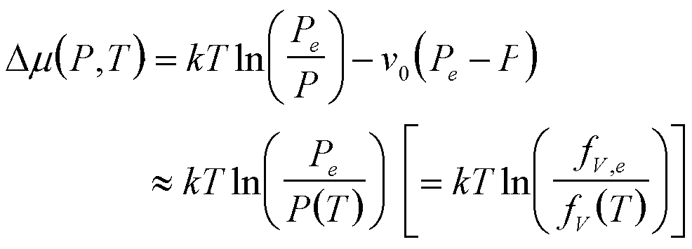
Supersaturation can occur due to any experimental parameter that can change the chemical potential of a material, so we can consider different types of homogenous nucleation depending on the parameter causing supersaturation and to some extent the phases which are in equilibrium and the direction of the transition, i.e. increasing or decreasing pressure for instance. What follows is a table of the expression for the chemical potential difference, the parameter effecting chemical potential and the name of the nucleation event.
| Name | Parameter(s) | Equation for Dm | Equation Number |
| Condensation | P, T |
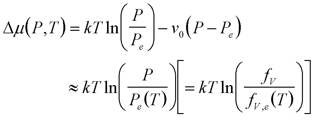 |
1 |
| Condensation of a Molecular Beam on a Surface |
I, T I = impingement rate |
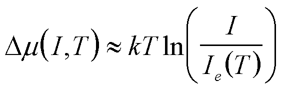 |
2 |
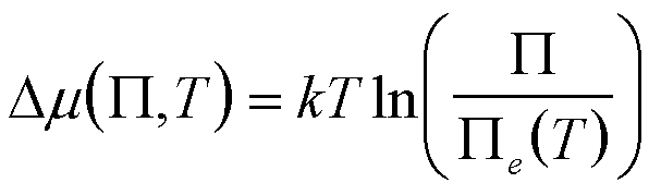
| Boiling | P, T |
 |
3 |
| Precipitation of a Single Component from a Liquid |
a (or f for dilute) |
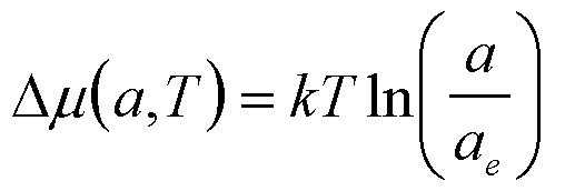 |
4 |
| Precipitation of multiple dissociating or reacting species under chemical equilibrium where m = ∑vimi |
P, T P = P aivi Solubility Product |
since generally viai/(vii,eai,e)
~ 1 except for a few species |
5 Nielsen 1964 Kin. of Precp. Sohnel Garside 1992 Prec., Bas. Prin. and Ind. Appl. van Leeuwen 1979 J. Cry. Gr. 46 91 and 96. |
| Dissolution into a liquid | P, T |
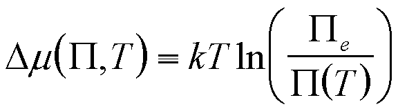 |
6 |
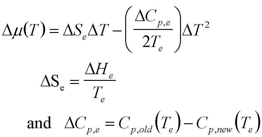
| Crystallization (or Polymorphic Transformation) |
T |
 |
7 |
| Melting | T (~Te) |
|
8 |
| Electrochemical Deposition | y, Galvanic
Potential |
zi = ion valence e0 = electronic charge |
9 |
| Electrochemical Dissolution | y |
 |
10 |
Homogeneous Nucleation and Clusters
Any material at a temperature higher than absolute 0 displays thermal fluctuations in the distribution of matter. This means that the density of the material varies randomly about the mean value observed for the bulk material. The size of these fluctuations in density varies depending on the temperature and transport properties of the atoms or particles that make up the material. Typically fluctuations occur on the 1 Angstrom to 1 nm scale for gasses, 1 to 10 nm scale for small molecules in the vapor state and at much larger scales, up to 10 micron for polymer melts for instance. These fluctuations can be thought to probe the P'/V' plot of Fig. 1 allowing a material to locally consider different densities and to compare the Gibbs free energy. Such fluctuations are not uniform in the system by definition since an increase in density requires and associated reduction in density in order to maintain an average density. Two main models have been proposed to calculate the free energy of formation of nuclei from a homogeneous system using the idea of fluctuations.
The simplest of these two models is the Gibbs cluster model which is the basis of most predictive equations for phase separation, Fig. 3 top. In the Gibbs cluster model an interface forms simultaneously with the formation of a cluster of elemental units. We can consider the free energy change on formation of the cluster by considering the number of elements in the cluster, n, and their free energy in the homogeneous phase as well as their free energy in the new phase which is discretely defined by the presence of an interface. The importance of the interface is that the energy of an element in the interfacial region is much higher than in the bulk of the cluster. Clusters grow larger in order to reduce their interfacial area per element and increase the bulk fraction of the cluster. By defining a pseudo equilibrium between a cluster of size n* and the homogeneous phase an equilibrium particle size can be obtained. In the Gibbs cluster model n* is generally smaller than 100 molecules.
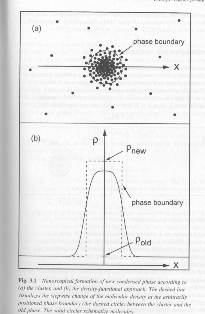
Figure 3.
The second model for formation of a nuclei is more recent and dates to the work of Cahn and Hilliard [1959]. The reason Cahn and Hilliard resorted to a new model for homogeneous nucleation is that cluster theory could not describe the earliest stages of nucleation in systems under a deep quench. For such systems many observations were made that a correlated web-like structure formed with a regular repeat distance between nucleii. Further, connectivity between the nucleii was observed. For such deep quench systems, early stage phase separation was not controlled by a balance between surface energy and bulk energy. In fact, Cahn and Hilliard proposed that a true interface did not exist and that the phase growth occurred directly from the dynamic features of the system, that is the structure of the composition fluctuations themselves. This model has come to be known as the density functional approach due to the involved mathematical functions that are necessary to describe the spatial and temporal distribution of density. Under some approximations, the density functional approach can describe all of the features of spinodal decomposition. Further, it offers a much more realistic view of nucleation at the price of fairly complicated mathematics. Under the density functional approach, phases initially grow not by local depletion of the homogeneous phase at the interface which drives Fickian transport, but by the nature of random thermal fluctuations themselves. Then transport of material to the growing nucleii, Fig. 3 bottom, occurs up a concentration gradient. Many other features of the density functional approach lead to unexpected predictions, most of which have been supported experimentally.
The phase size using the density functional approach will be related to the square root of the elemental diffusion coefficient times the size of the elements divided by the quench depth in terms of the difference in the chemical potential with the spinodal chemical potential. Phases with a significant distribution in size are predicted with the square of the maximum probability phase size being twice the square of the critical size. The diffusion coefficient occupies a similar relation with size that the surface energy takes in the Gibbs cluster model. Then the density functional approach is essentially a steady state dynamic model. The absence of a true surface is compensated by the kinetics of transport of the elemental units that are thermally driven. A simpler approach might be to directly consider that the interface of a nano- to atomic phase is not the same as the interface of a bulk phase in that it generally displays a gradient that is much broader relative to the phase size. The breadth and energy cost of this interfacial region is governed by Fickian diffusion.
Gibbs Cluster Model
The work to form a cluster of size n, W(n), is given by,
W(n) = -nDm + Gex(n) (11)
where Gex is the excess energy associated with the cluster (surface energy etc.). For clusters of condensed phases (precipitation for instance) Gex is the cluster total surface energy, f(n). For clusters of gas phases Gex is given by,
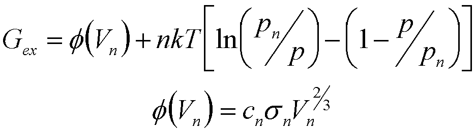 (12)
(12)
For a liquid or solid phase Vn is related to n directly and,
 (13)
(13)
For nucleation of a gas phase the generalized Laplace equation can be used to calculate the pressure in the cluster,
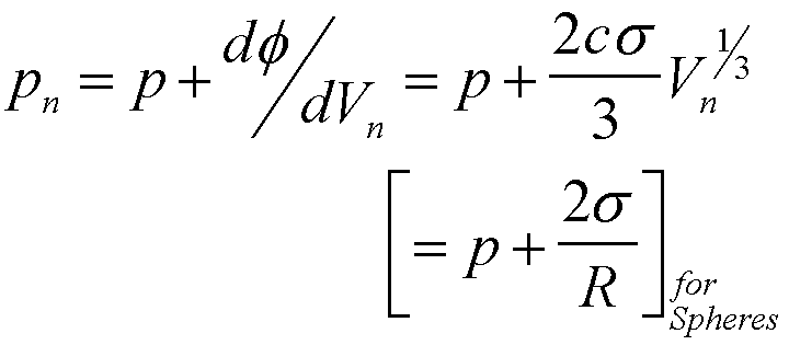 (14)
(14)
Using the ideal gas law and Eq. (14) it is seen that there is no simple functional form for f(n) since the relationship between Vn and n is complex,
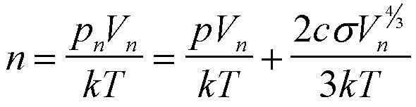 (15)
(15)
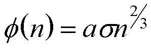
With this in mind several expressions for Gex can be written,
| Independent Parameter |
Liquid or Solid Precipitate |
Gas Nucleus |
| Gex(Vn) | csVn2/3 |
 |
| Gex(n) | asn2/3 |
 |
| Gex(R) | 4psR2 |
 |
The work of nucleation from eq. (11) is listed in the following table,
| Independent Parameter |
Liquid or Solid Nucleation |
Gas Nucleation |
| W(Vn) | -(Dm/v0)Vn + csVn2/3 |
 |
| W(n) | -nDm + asn2/3 |
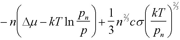 |
| W(R) | -(4pDm/3v0)R3 + 4psR2 |
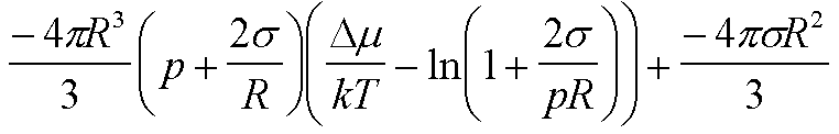 |
Figure 4 shows the behavoir of W(n) for water homogeneously nucleating liquid droplets from vapor (condensation) and vapor droplets from liquid (boiling). The more complicated functions for vapor nucleation lead to a broader work plot with a higher energy barrier and a larger critical nucleus, n*.
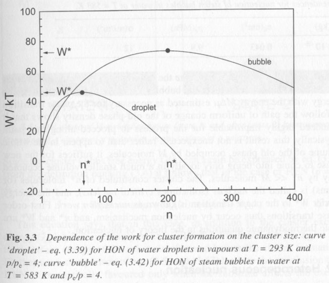
Figure 4.
In figure 4 it is seen that a critical size is reached, dW/dn = 0 where the energy barrier to nucleation is a maximum and where, beyond this size particles will reduce the work to form nucleii by growing larger nucleii. This is the minimum size for a stable nucleus. The work function, which is a balance between the surface and bulk energies in the Gibbs cluster model, also passes through 0 where the surface and bulk properties just balance. The table below shows values for W*, n*, p*, and R* for spherical nucleii.
| Parameter | General | Liquid Nucleii | Gas Nucleii |
| W* | W(n*) or -(p*-p)V* + fs* | 4c3vo2s3/(27Dm2) | 4c3s3/(27kT(p*-p)2) |
| n* | n at dW/dn = 0 | 8c3vo2s3/(27Dm3) | 8c3p*s3/(27kT(p*-p)3) |
| p* | p + (dfs/dVn)* | p + 2cs/3 V*1/3 or pe exp(-v0Dp/kT) | |
| R* | 2v0s/Dm
(sphere n* = 32pvo2s3/(3Dm3) |
2s/(p*-p) (sphere n* = 32pp*s3/(27kT(p*-p)3) ) |
Figure 5 shows the behavior of n*, R* and W* versus Dm for homogeneous nucleation of water droplets from vapor.
Figure 5.
Cluster Properties:
| Property | condensed | gas |
| pn | p + 2sn/R + dsn/dR p + 2cs/3 vo1/3n1/3 |
p + 2cs/3 Vn1/3 |
| mnew,n | mnew(p) + 2svo/R | mnew(p) + kTln(1 + 2s/pR) |
| pe,n | pe exp(2svo/kTR)
Kelvin for spheres or for variable sn pe exp((vo/kT)(2sn/R + dsn/dR) |
pe exp(-2svo/kTR)
Kelvin for spheres or for variable sn pe exp(-(vo/kT)(2sn/R + dsn/dR) |
| Ce,n Solubility | Ce exp(2svo/kTR)
Kelvin for spheres or for variable sn Ce exp((vo/kT)(2sn/R + dsn/dR) |
|
| Te,n Melting Point | Te - (vo/Dse)(2sn/R
+ dsn/dR) Spherical Crystallites |
|
| sn | s/(1 +
d0/R)2 if R >> d0 s exp(-2d0/R) n-dependence s/(1 + cd0/(3n1/3vo1/3))2 d0 is believed to be on the order of molecular diameter but sign is not known (a guess is +0.1 nm) |
Complex form |
Figures 6 and 7 show these dependencies for water droplets and water vapor bubbles.
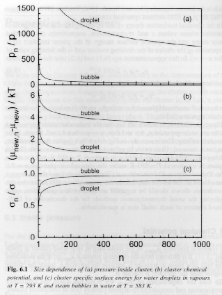
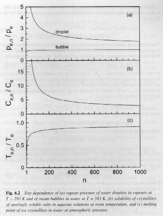
Figures 6 and 7.