X-Ray Diffraction Lab

X-Ray Diffraction Lab Experiment 2

Pinhole/Polaroid Diffractometer

Download Data: UHMWPE.gif, Azimuthal Averaged Data.MSExcel, Radial Averaged Data.MSExcel, Al Foil 6.75 cm SDD, Fishing Liscense 3.8 cm SDD, PE 3.8 cm SDD, PE Recryst 3.8 cm SDD, PE Stretched 6.75 cm SDD, PE Bag 3.8 cm SDD, PET Bottle Amorphous (as processed) 3.8cm SDD, PET Bottle, Recrystallized 3.8 cm SDD, View Pinhole Photos

Objective: To become familiar with operation of a 4kW Philips x-ray generator and to look at some simple 2D-XRD patterns in processed materials using a Polaroid film.

Background: Cullity pp. 175 (Chapter 6), pp. 281 (Chapter 9), pp. 358 (Chapter 11). R. J. Roe Methods of Neutron and X-ray Scattering in Polymer Science Chapter 3.

A pinhole diffraction experiment using photographic film or a Polaroid camera is probably the simplest approach to observation of crystalline diffraction using x-rays. Figure 6-11 on page 175 demonstrates the type of diffraction pattern which can be obtained using this technique. If orientation is important it is critical to note the arrangement of the film with respect to the camera and sample. You should make a careful record in your notes on the orientation of the film with respect to the camera and of the orientation of the sample in the camera.

The pinhole technique involves pinhole collimation of the beam as opposed to a line beam. The x-ray tube typically has four ports from which x-rays can be obtained. The footprint of the electrons from a linear filament will be a line on the anode (Cu in this case). From two of the ports a line beam is produced and from the other two a point beam is produced. It is best to choose the point source if pinhole collimation is to be used since this will result in higher flux. The beam which is produced from the generator is from about 2 mm to less than 1 mm depending on the size of the filament (i.e. normal or micro-filament). Finer filaments produce better collimation but tubes with fine filaments burn out faster. For pinhole collimation it is the size of the beam which determines the angular resolution which can be obtained.

The pinhole technique is an extremely useful and cheap technique for screening samples especially for processed materials. Alignment of collimation is simple and can usually be achieved in less than an hour. The beam from the Cu target is attenuated with a sheet of Nickel to reduce the beta peak. You should make sure to note the voltage and current at which the generator is operated during the experiment as well as estimating the power for the generator

The pinhole technique is a fairly simple lab which is intended to demonstrate diffraction from common materials. We will examine oriented and unoriented samples of polycrystalline aluminum, polyethylene and some fibers to investigate fiber patterns. For the processed samples we will perform a crude estimate of the orientation function to describe orientation effects. The crystalline d-spacing and verification of the diffraction indexing will also be performed. An estimation of the crystalline size will also be performed for the PE samples from image plate data which will be supplied.

It is possible to obtain quantitative data in a diffractometer arrangement identical to the photographic pinhole camera used in this lab. This can be done using a 2-D wire detector or using an image plate detector. A 2-d image plate pattern from polyethylene will be provided on the web. This image has been averaged azimuthally and radially at specified values of 2-theta corresponding with some of the diffraction peaks. The excel files for the averaged data are also included on the web.

(Links to PE crystal structure on the web: Darmstadt)

Polyethylene samples typically contain some inorganic processing aids, typically silica (SiO₂) which is usually in an a-quartz crystal structure, hexagonal with a = 4.9136Å and c=5.40512Å. It is easy to identify these inorganic additives in the diffraction pattern since the polymer crystals are very small and give rise to smooth Debye-Scherer rings with significant breadth, while the inorganic processing aid gives rise to a grainy pattern with no orientation and a fairly sharp band, see figure 9-1 pp. 283.

Polyethylene crystallizes in an orthorhombic crystalline structure (Lab 2) with lattice dimensions of a=7.40Å, b=4.93Å and c=2.534Å. The c-direction is the chain direction. Typically only three strong reflections are observed, (110), (200) and (020), with the (200) being the prominent peak. These peaks are superimposed on a broad region of intensity which results from the amorphous component of the polymer (polymers are usually not 100% crystalline). This amorphous halo reflects a preferred spacing of PE chains in the amorphous state. Typically, polymer samples display significant intensity at very low angle which reflect colloidal scale structure associated with stacked lamellar crystallites. The pattern at very low-angles, 0.01° to about 6° can be analyzed using various approaches of small-angle scattering.

The breadth of the diffraction peak is related to the size of the crystals by the Scherer equation which we will derive in class. The measurement of the breadth of the diffraction peak and calculation of the crystalline size using the Scherer equation is a primary method to determine crystallite dimensions. The Scherer equation is given on pp. 284 in chapter 9 and is derived earlier in chapter 3 of Cullity and . The size of a crystallite, t, giving rise to a diffraction is inversely proportional to the breadth of the peak, B, in radians. The peak breadth can be estimated from the photographic image simply by measuring it off the pattern and converting this number to radians.

t = 0.9 l/(B cosq)

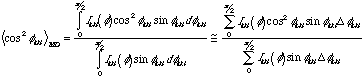
where l is the wavelength and q is half the angle of diffraction (2q). Typically the half-width at half-height of the diffraction peak is used for B which can be estimated as half the peak width on the diffraction photograph. A careful consideration of the error in this method using the photographic method should be made. Usually, the Scherer method is applied to diffractometer traces which we will look at in a later lab.

A quantitative estimate of the degree of orientation in a processed sample can be obtained through calculation of the Hermans orientation function, f_hkl. The Hermans orientation function can have values in the range -0.5 to 1. A value of -0.5 indicates that the crystalline planes are oriented perpendicular to the machine direction, a value of 0 indicates random orientation and a value of 1 indicates perfect orientation in the MD. For an orthogonal crystal the Hermans orientation function for the three unit cell axes sum to 0. The Hermans orientation function for a given plane can be calculated by calculation of <cos²f> where f is the azimuthal angle in a 2-d pattern such as you will obtain in this lab. The Hermans orientation function can be used as a weighting fraction in calculation of properties of a material in the various sample directions, i.e. modulus in the MD and CD directions for a blown film.

Estimation of Hermans Orientation Function. Using the image plate data (radial averages) that displays orientation you the intensity as a function of f for a fixed 2q_hkl on prominent diffraction peaks has been obtained, (200) for PE for instance. f=0 is in the MD direction. <cos²f_hkl> is determined by:

(1)

The orientation function is directly calculated from <cos²f_hkl>,

(2)

Aluminum has a FCC structure with a=4.0497Å. Figure 9-11 displays a pinhole diffraction pattern from an aluminum wire with the (111) and (200) reflections being the most prominent. Notice that the edge of the photograph has been marked by cutting the top right edge for identification of the camera orientation.

If time permits you can run diffraction patterns on other samples of your choice. Make sure to keep careful notes on these and to include them in your lab reports. Samples might include other fibers, salt, amorphous plastic pieces etc.

Specific issues to be addressed:

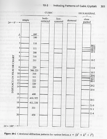
1) For all samples calculate 2q, d_hkl, and identify the planes which give rise to all strong reflections (about 3-4 per sample). If you see silica in the PE pattern verify
that this is quartz by the same calculation.

2) For the polymer samples estimate the crystalline size using the Scherer Equation. (You might also try this for the aluminum samples).

3) Calculate the orientation function for the image plate data as described above. In your discussion list the three limits to the orientation function and the values of f
and <cos²f> for these cases. Describe the usefulness of the orientation function.

4) Discuss the differences in appearance between polycrystalline metal patterns, polymer and ceramic (silica in terms of Figure 9-1 on pp. 283). Also discuss why
the silica in PE doesn't orient while the PE reflections can become highly oriented. (This pertains to the shape of polymer crystals vs. the shape of silica grains).