Vector and Tensor Mathematics
![]()
Mathematics for Modeling
The intent of this section is to give a refresher in vector and tensor mathematics, a critical tool for modeling any system.
What is a vector?
A vector is a physical representation of a physical quantity that possesses both magnitude and direction. Examples of vectors are forces acting on a body and velocities of objects. A vector can also be thought of as a first order tensor…a term that will be explained later. To envision a vector, one pictures an arrow pointing in the direction of the vector and having a length representative of the magnitude of the vector. Vectors can be classified into subcategories which include:
|
Equal vectors: two vectors having the same magnitude and direction | |
|
Unit vectors: a vector of unit length and is calculated by dividing the vector by its own magnitude | |
|
Null or Zero vectors: a vector with zero magnitude (zero length) and an unspecified direction | |
|
Negative vectors: two vectors having the same magnitude, but opposite directions |
Under symbolic (also called Gibbs)
notation, vectors are designated by bold-faced letters and scalars are
denoted as italic letters. Unit vectors are typically represented with a
caret placed over a bold-faced letter (![]() ).
The magnitude of the vector can be represented by its scalar value, a, or
by placing the vector symbol between vertical bars, |a|.
).
The magnitude of the vector can be represented by its scalar value, a, or
by placing the vector symbol between vertical bars, |a|.
Vector Addition
Vector addition is easily visualized with the parallelogram law or triangle rule, as shown below:
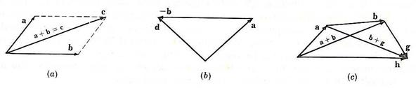
image: Mase, G., Schaum's Outline of Continuum Mechanics, 1st edition, McGraw-Hill, 1969.
The parallelogram law states that the sum of two vectors is represented by the diagonal of a parallelogram having the component vectors as adjacent sides. An alternative technique, the triangle rule, states that the sum of the two vectors is represented by the vector extending from the tail of the first vector to the head of the second vector when the vectors to be summed are adjoined head to tail.
Multiplication of a Vector by a Scalar
When a vector is multiplied by a scalar, the resulting product is simply a new vector with the same direction, but a different magnitude. The following figure shows the result of the multiplication of a vector, b, by a scalar, m, of various magnitudes.
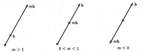
image: Mase, G., Schaum's Outline of Continuum Mechanics, 1st edition, McGraw-Hill, 1969.
Dot and Cross Products of Vectors
The dot product of two vectors results in a scalar (magnitude without direction) value and is calculated by multiplying the magnitudes of the vectors and the cosine of the angle between the two vectors.
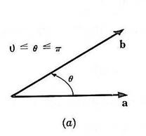
image: Mase, G., Schaum's Outline of Continuum Mechanics, 1st edition, McGraw-Hill, 1969.
a∙b = b∙a = abcosq
Two uses of the dot product are to:
determine the angle between two vectors
determine the projection (P) of a one vector onto another such that the projection of a onto b is:
The cross product of two vectors results in a vector (magnitude and direction) value and is calculated by multiplying the magnitudes of the vectors with the sine of the angle between the two vectors and the unit vector that is perpendicular to the plane with which vectors a and b lie.
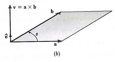
image: Mase, G., Schaum's Outline of Continuum Mechanics, 1st edition, McGraw-Hill, 1969.
axb = -bxa
= (absin(q))![]()
The angle
q is determined by the angle that is less than 180 degrees that a
right hand rotation about ![]() brings
a into b. The magnitude of the cross product is equivalent to the
area of the parallelogram that has a and b as adjacent sides.
brings
a into b. The magnitude of the cross product is equivalent to the
area of the parallelogram that has a and b as adjacent sides.
When both cross and dot products are present in a single multiplication, the cross product must be carried out first, then followed by the dot product.
Invariants are functions of vectors that are independent of a coordinate system. To explain, lets consider the velocity of a point mass, which is a vector and is proportional to its kinetic energy.
![]()
Kinetic energy is not a vector...it is a scalar with only a magnitude (no direction), but the velocity is a vector. This issues is explained by the fact that there is a scalar function of the velocity, given by:
![]()
![]()
![]()

![]()
![]()
![]()
Coordinate Systems including Base Vectors and Unit Vector Triads
The choice of a coordinate system is purely arbitrary, and should be established to the greatest advantage of the problem.
The coordinate set to be discussed, and most commonly used, is the rectangular Cartesian system.
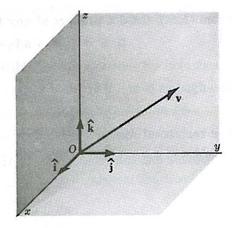
image: Mase, G., Schaum's Outline of Continuum Mechanics, 1st edition, McGraw-Hill, 1969.
This system is most commonly represented by mutually perpendicular axes (Oxyz), shown in the above figure. Any vector within this system (v) can be represented by a linear combination of three noncoplanar vectors (also known as the base vectors represented by a, b, and c).
v = la + mb + nc
Another notation, and one commonly
seen for rectangular Cartesian systems, uses a set of unit vectors consisting of
![]() .
This notation will be used for the remainder of this discussion on vectors. The
vector in terms of this orthonormal basis is represented by:
.
This notation will be used for the remainder of this discussion on vectors. The
vector in terms of this orthonormal basis is represented by:
The following relationships are obtained by breaking out each directional component of the vector relative to the angles between the vector and the Cartesian axes shown in the following figure:
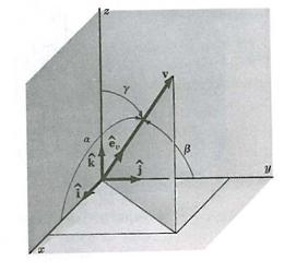
image: Mase, G., Schaum's Outline of Continuum Mechanics, 1st edition, McGraw-Hill, 1969.
vx
= v∙![]() =v
cosa
=v
cosa
vy
= v∙![]() =v
cosb
=v
cosb
vz
= v∙![]() =v
cosg
=v
cosg
The dot product of two vectors represented in the Cartesian component notation is given by:
a∙b = axbx+ ayby+ azbz
The cross product of two vectors represented in the Cartesian component notation is given by:
axb = (aybz
– azby)
![]() +
(azbx – axbz)
+
(azbx – axbz)
![]() +(axby
– aybx)
+(axby
– aybx)
![]()
Which is often presented in the determinant form:
axb =
To this point, we have only discussed rectangular Cartesian coordinate systems, but vectors can also be expressed in cylindrical (R, q, z) and spherical (r, q, f) terms, as shown in the figures below.
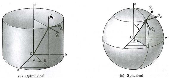
image: Mase, G., Schaum's Outline of Continuum Mechanics, 1st edition, McGraw-Hill, 1969.
What is a Tensor?
A tensor consists of a set of quantities that obey certain transformation laws relating the bases in one generalized coordinate system to those of another and involving partial derivative sums. Vectors are an example of simple tensors. Tensors depend linearly on several vector variables and vary covariantly with respect to some variables and contravariantly with respect to others when the coordinate axes are rotated. Tensors are used in a wide range of scientific fields, including the study of relativity, fluid mechanics, elasticity, plasticity, viscoelasticity, strength of materials, and continuum mechanics. For example, tensors are used to express the differential permeability of organs to water in varying directions to produce scans of the brain. The most commonly know tensors for engineers are the strain tensor and stress tensor (both 2nd rank tensors), and are related by the elasticity tensor (which is fourth rank).
An nth rank tensor in m-dimensions is a mathematical object that has n indices and mn components and obeys certain transformation rules. For example, in three-dimensional Euclidian space (as we are most accustom to thinking about), the number of components of a tensor are 3n, where n is the order of the tensor. Tensors are generalizations of scalars (that have no indices or an order of zero), vectors (that have exactly one index or an order of one), and dyadics (that have exactly two indices or an order of two) to an arbitrary number of indices (progressing through triadics, tetradics, etc.). Several important quantities in mechanics are represented by these tensor of rank two (dyadics), so the following section will focus on the mathematics associated with these second order tensors.
Coordinate Transformations-the Basis of a Tensor
First, we let xi represent an arbitrarily chosen set of coordinates (x1, x2, x3) in our familiar three-dimensional Euclidian space. Next we define qi as any other coordinate system in the same space (q1, q2, q3). One must be careful not to confuse the superscripts, which serve as notations, with the term raised to a given power. Now we can define the coordinate transform equations as:
![]()
This relationship allows us to assign a new set of coordinates in the (q1, q2, q3) system to any point in the (x1, x2, x3) system.
The determinant, called the Jacobian on the transformation, is given by:

If the Jacobian does not vanish, the previously mentioned coordinate transform equation has a unique inverse set, given by:
![]()
This inverse property means the two coordinate transform equations are completely general and may be curvilinear or Cartesian system.
Application of Tensors in Continuum Mechanics
Tensors are mathematical objects that are independent of coordinate systems that are used in continuum mechanics to provide computational convenience. Three areas where tensors are extremely helpful are:
|
Constitutive Relationship between Stress and Strain (combining the first two items)…see the web page on continuum mechanics. |
Since we have already mentioned the stress tensor, we can now derive equations of equilibrium that govern its components.
First, we define a body force vector per unit volume (f) that is acting upon a body and the vector force per unit area acting on a surface (F). For any volume (V) bounded by surface (S), equilibrium requires that:
![]()
For an arbitrary system with curvilinear coordinates, we redefine f and F as:
f = fjej
F = Fjej = sijniej
Next, by defining N=Niei as the unit outward normal to the unit surface area at which the force is acting and substituting the equations for f and F into the previously mentioned equilibrium equation, we obtain:
![]()
Next we apply the previously described divergence theorem, we obtain:
![]()
Since this equation holds true for all volumes (V), and since ej;i = x;ji = 0, then:
sij;i + fi = 0
It is also worth noting that since the net momentum of the body must vanish, sij = sji.
In most modeling efforts of polymer processing, a key parameter that must be characterized and understood is the deformation of the material and how it relates to the applied displacement and strain. To begin this section, let’s envision a coordinate system in the body (x1,x2,x3) and a vector in that coordinate system, x(x1,x2,x3) to denote the position of that material after it has been displaced from its original position, noted as x0(x1,x2,x3). At this point, it is important to clarify that these are convected coordinates, meaning that they are engraved on a moving body, as we will see as a polymer bubble in the blown film modeling section.
The displacement vector, U, is calculated by taking the different between the displaced position vector and the original position vector:
![]()
While studying stress, we will define the base unit vectors for the deformed body as:
![]()
In some cases, it is easier to envision the displacement vector relative to the undeformed body, which is defined as:
U = uie0i
where the base vector is defined as:
![]()
Since the two geometries (undeformed and deformed states) have different metric
tensors, we can write the following for our dynamic, deforming system:

It should be noted that the metric tensor is used to relate two kinds of components for any given set of general base vectors. For example:
Fi = gijFj
At this point, the Lagrangian strain tensor (hij) can now be defined as a measure of the deformation, and is given by:
![]()