Introduction to Continuum Mechanics

In this section we will present the concept of continuum, discuss stress in a continuum and those factors that affect it, dynamic and continuity equations, kinematic, and constitutive equations.  The knowledge gained in this section will later be used in an example that presents constitutive equations describing the flow of viscoelastic fluids.

What is Continuum?

A continuum, or continuous medium, is a region defined in space where various properties, such as temperature, pressure, density, and velocity, may vary in a continuous manner.  Some examples include the section of a blown film bubble, a defined volume of a polymer/solvent solution, or a portion of a polymer melt as it passes through an extruder, feed block, and die.

To elaborate further on each of these examples, we study how various properties change as a result of the effects of the process on the continuum.  In the first case, the molten polymer exits the die and is initially drawn in the machine (vertical) direction.  At this point, we have changes in temperature and density as a result of the hot polymer being cooled by the air ring and crystallization occurring, and velocity in the machine direction as the tube is drawn.  At a specified height, the tube is blown up in the transverse (horizontal) direction…introducing a second change in velocity with the continuation in cooling and crystallization.  In the second example, we could experience changes in concentration (density) if the temperature is reduced.  If the solution was stirred, changes in velocity would also occur.  In addition, if a reaction were to occur, changes in temperature, pressure, and concentration would be evident.  In the final example, changes in temperature are the result of shear and external heat from the extruder and die heaters. 
As the polymer is extruded, changes in velocity and pressure are evident, with decreases in density occurring as the polymer is melted.

As one can see, these properties are not only changing, but are interrelated and in some cases, controlled by the conditions of the process.  It is the job of the engineer to understand the dynamics and those parameters which can be affected to optimize any process.

Stress in Continuum

When attempting to characterize the stresses acting on a fluid, the first task is to understand the various forces action on that fluid.  Some examples include forces from motion (say from agitation), body forces (i.e. gravity), viscoelastic effects, or pressure distribution.

Once we understand the various forces, we then define an area (DA).  Note the bold font of the “A”.  If you recall from the section on vectors, both the magnitude and direction of the entity are given.  In this case, both the magnitude as well as the direction (i.e. the orientation) of the area is critical.  The directional component of the area vector is given relative to its normal vector, n.  The force acting on the specified area (DF), is also a vector having different direction than n, as indicated in the following figure

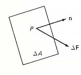
image: Middleman, S., Fundamentals of Polymer Processing, 1^st edition, McGraw-Hill, 1977. 

The next step is to resolve the force vector (DF) into components relative to a cartesian coordinate system consisting of n, s₁, and s₂, where s₁ and s₂ are surface axes of the specified area.  The components of the force vector are then noted as DF_1n, DF_2n, and DF_3n.  At this point, we need to clarify the double subscript notation.  Since we can choose an infinite amount of areas, each with their own “n” normal vector, the second subscript is indicative of which “n” vector that represents the area we are characterizing.  This second subscript is indicative of the orientation of the area relative to an external, predefined coordinate system (say the machine, transverse, and noral directions of a film) and can also be thought of as the “surface” relative to which the force is acting upon.  The first subscript is simply indicates which axis (n, s₁, and s₂) the force vector has been resolved to.

Now that the components of the stress vector have been defined, we can express the stress vector at a given point in the predefined area (relative to a given axis for a specific n vector) as:

The following figure shows the resolution of a force acting upon a body:

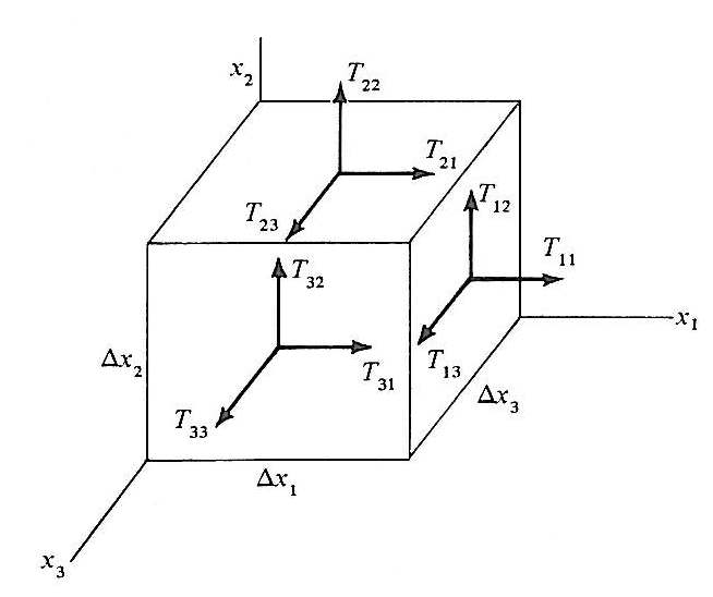
image: Malvern, L. E., Introduction to the Mechanics of a Continuous Medium, Prentice-Hall, 1969.

At this point we must also define the sign of the force acting on each surface in a defined direction.  All forces shown in the above figure are positive.  This means that a force is positive if the normal force pulls to the right on the right side of the block and pulls to the left side on the left side…i.e. a tensile force.  When the force is negative, the stress is compressive.

We will also make the statement that if the nine components of the force are know for a specific set of axes, then the components for any given normal resulting in an alternative set of axes can be determined.  We won’t go into great detail discussing this section, but Malvern (p. 73-77), Fung (p. 70-72), and Middleman (p.16-19) discuss the Cauchy’s tetrahedron, with Middleman deriving the relationships between alternatiave normal vectors in terms of cosines of the angles between the defined axes.  Such a relationship that transposes from the ij coordinate system to the kn system is given by:

Where the prime (‘) indicates the stress relative to an axis in the alternative normal coordinate system (k) relative to the normal of the original coordinate system (n).  The k term is indicative of an axis in the alternative coordinate system (k = n’, 1’, or 3’).  The i and j terms are indicative of a direction (i) relative to a plane (j) in the original coordinate system.  The a term is simply the cosine of the angle between the subscripted axes.

Since the nine components (T_ij) are sufficient to define the state of stress at any given point in the continuum, it is now convenient to define the stress tensor, noted as T.

A common assumption in continuum mechanics is that the stress tensor is symmetrical, meaning that:

For a clarification of the argument regarding the symmetry of the tensor, one is referred to Middleman (p. 18), which describes the effects of symmetric stress components on a parallelepiped.  Simply stated, each force generates a moment about a common axis equal, but opposite in magnitude to its counterpart.  Next, assuming body forces (i.e. effects of gravity) and angular momentum are much less than that of the tensor component, momentum is conserved and the symmetrical tensor components are equal.  Some care should be taken in making this assumption.  Systems that are intrinsically asymmetric might show asymmetric tensor components.  These systems include liquid crystals or dispersed asymmetric materials in a matrix.  This assumption means that only six of the nine components of the tensor are necessary and allows for simplification of the mechanics problems.

Dynamic and Continuity Equations

In this section, we will derive two basic conservation equations:

Continuity Equation

To derive the continuity equation, we first define our system as the following:

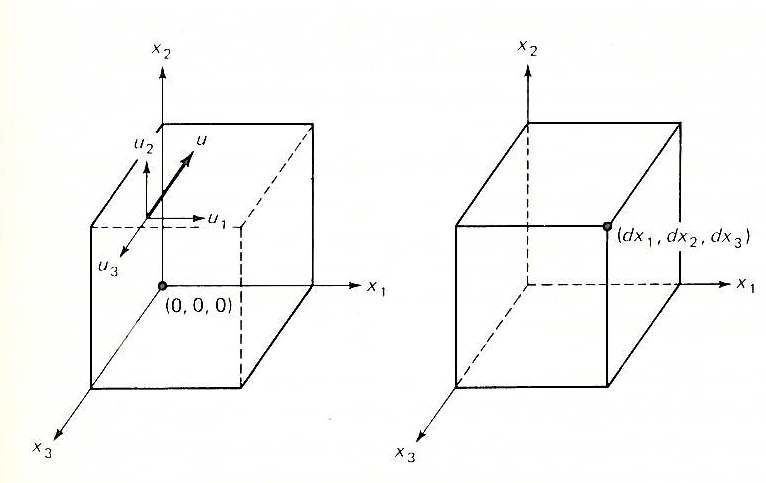
image: Middleman, S., Fundamentals of Polymer Processing, 1^st edition, McGraw-Hill, 1977. 

Where we have two parallelepipeds, the first representing an initial state with the second representing the differential state.  The volume of the parallelepiped has a differentially small volume of magnitude:

The net rate of change of mass within the volume is now given as:

Next, the volumetric flow rate across a surface is given by the product of the surface area and the velocity normal to that surface:

Now, if we consider two parallel surfaces perpendicular to the x₁ axis, the net flow across the pair of faces is given by:

To simplify the notation, we introduce the following definition, which represents a function of the net flow as a function of both time and position.

Substituting [F_i] into the net flow equation gives the following relationship:

Which can be solved with a Taylor Series expansion to yield:

In reality, there are three of these net flow equations, where i=1, 2, 3.  Combining these three equations and disregarding the higher order terms in the spirit of simplification, the total time rate of change of mass within the chosen volume element (i.e. ), is:

If we substitute the previously mentioned definition of [F_i] and divide out the volume, we obtain:

For a very small volume element (dV→0), the above equation gives the mass balance in an infinitesimal neighborhood about a point centered in dV.  This means the terms of order dx vanish and the final continuity equation for a compressible fluid is:

For an incompressible fluid, the final continuity equation is:

With this notation,  is the divergence operator and u is the velocity vector.

Dynamic Equations

Now, to derive the dynamic equations, we have to build a relationship for the conservation of momentum that includes terms for applied stresses, body forces, deaccellerat and, deconvection.

Stresses

Let us consider a region of a continuum subject to stresses which may vary continuously throughout the small volume dV.  The following figure shows these stresses:

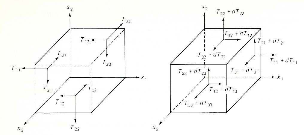
image: Middleman, S., Fundamentals of Polymer Processing, 1^st edition, McGraw-Hill, 1977. 

The stresses in the first set of planes, represented by T_ij, are varied in the second set of planes by a delta equivalent to dT_ij.  We can write the stresses on a given plane in the varied (or second) set of planes in terms of the stresses see in the original set of planes by using a Taylor Series expansion to give:

Now, taking into consideration the forces illustrated in the above figure and dropping the higher order terms from the Taylor Series for simplification, we can write an equation for the net x₁ component due to stresses (S₁) as:

As you can see, there are three of these equations, with the other two for S₂ and S₃.

Body Forces

Body forces, which are those typically associated with gravity and are proportional to the mass of a body, must also be accounted for.  If we take f₁ as the component of the body force in the x₁ direction, then the body force component becomes:

Acceleration

The acceleration term is simply the change in momentum density with respect to time, or:

We talk in terms of a momentum density since we normalize the factor about a unit volume.  If the element under consideration is a rigid body, we only need the stress and body force components to satisfy Newton’s second law.  Typically, the volume being studied in polymeric systems are not rigid, and in essence, are a fluid.  For fluid systems, material is allowed to cross the boundaries of the system, which must now be accounted for in a convection term.

Convection

If u is the velocity vector of the volume element, any amount of fluid crossing a surface of the control volume has a momentum per unit volume (momentum density) of ru.  To calculate the rate at which momentum crosses a surface, we simply multiply the density of momentum by the velocity with which the fluid crosses each surface.  So the x_i momentum flow into face dx_jdx_k is:

As you know, there are three of these equations, one each for the i, j, and k component of the momentum density into their respective normal face.  Again, a Taylor Series is used and the net flow of x_i directed momentum across all six surfaces of the control volume is represented by the convective terms, and is given by:

Combining it all…

Now, we combine all of the previously derived terms to get a general equation for the momentum principle for the volume element, which is:

Next, we divide both sides of this equation by dV and take the limit as dV→0.  We assume that the differential terms remain finite and well behaved (i.e. no discontinuities).  This yields the dynamic equation for a continuous medium, which is:

Again, as one can see, there are three equations where i = 1, 2, and 3.

Now, substituting in the continuity equation that we previously derived and assuming that mass is conserved, we obtain:

In this format, the dynamic equations are known as Cauchy’s stress equations.

The following table shows the dynamic and continuity equations for various geometries, including cartesian, cylindrical, and spherical geometries.

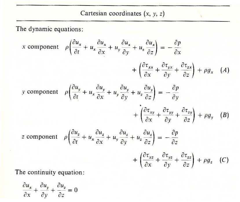
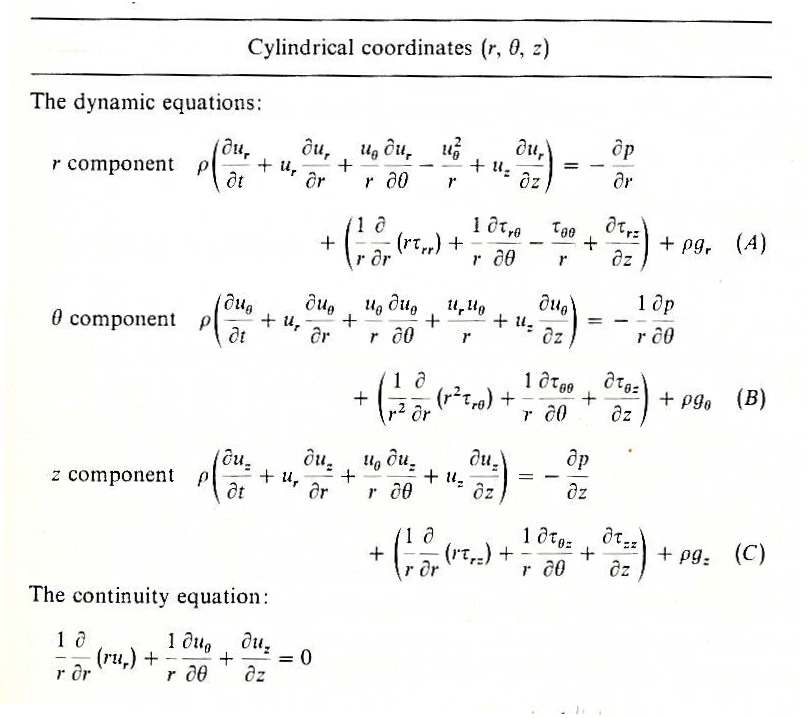
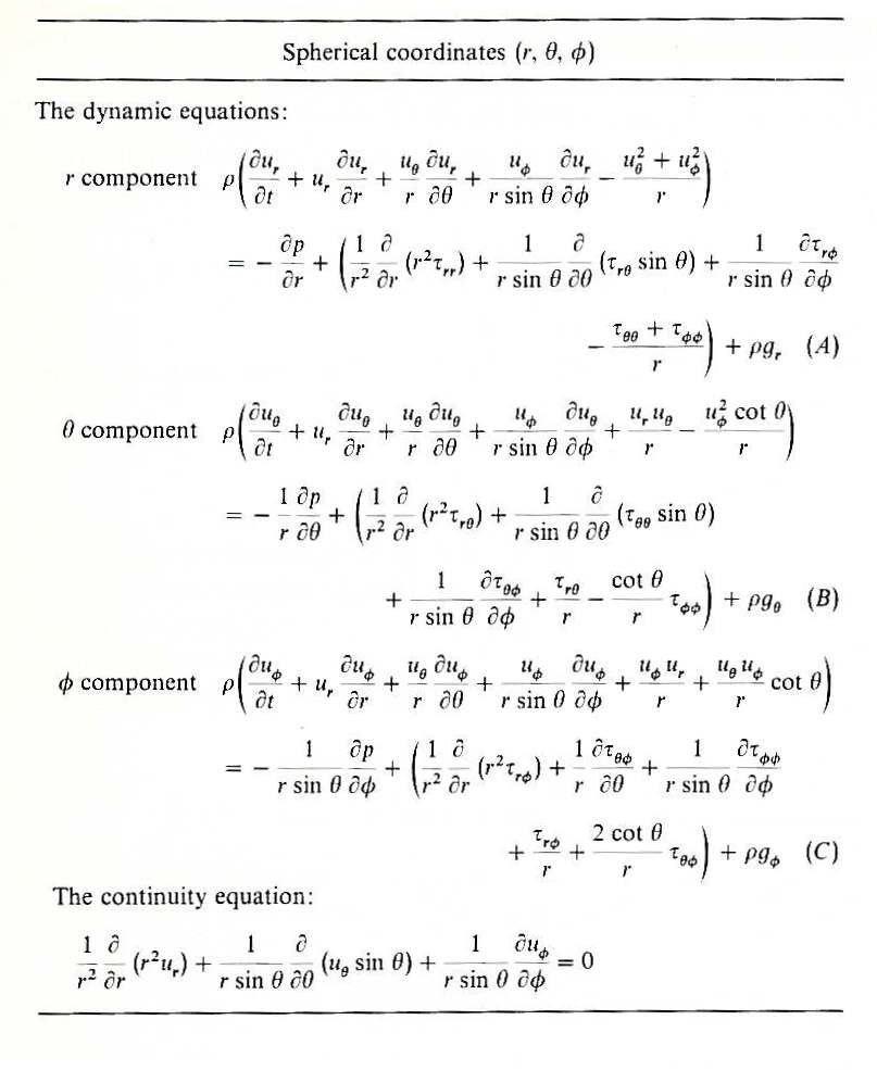
image: Middleman, S., Fundamentals of Polymer Processing, 1^st edition, McGraw-Hill, 1977. 

Kinematics

Kinematics refers to the analysis and description of motion of an object through space.  It differs from dynamics in that dynamics is interested in relating the motion of an object to the force that is causing that motion.  If we consider a continuous medium that is in motion characterized by the vector u, which has components u_i, u_j, and u_k, we can express the components of the velocity in the volume near a reference point (with the reference point noted by the subscript 0) by a Taylor Series as:

Decomposing the velocity gradient into two parts results in the following:

If we define:

Upon examination of the first term (w_ij), we find that it is simply a rigid rotation depending on the w_ij term (See Middleman p. 28 for details).  The second term (D_ij) is the rate of deformation tensor and in the case of many materials, the stress components (T_ij) depends only on this term.  Simply stated, it is this rate of deformation term that connects the dynamics and kinetics of the motion of a fluid.  The following table lists the rate of deformation tensors for cartesian, cylindrical, and spherical coordinates.

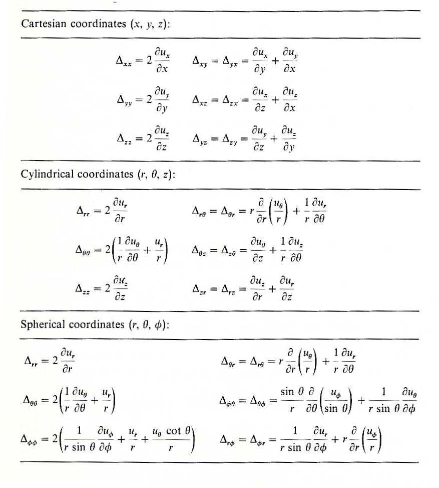
image: Middleman, S., Fundamentals of Polymer Processing, 1^st edition, McGraw-Hill, 1977. 

Constitutive Equations

The dynamic equations capture the conservation of momentum and relate the velocity (u) vector to the stress tensor (T).  These equations are true for any fluid for which continuum approximations are meaningful, which means they are not concerned whether the fluid is newtonian or non-newtonian, or viscoelastic or elastic.  The continuity equation is strictly a kinematic constraint among the velocity gradients and gives no information regarding the stresses, and thus the type of fluid (except for compressibility).    Based on these statements, one wonders where the mechanical constitution of the fluid enter into the process model?  This is where the constitutive equations enter the analysis.  They relate the components of the stress tensor to the kinematics, by utilizing D, and thus define the type of fluid that is being modeled.  Their purpose is to provide additional equations so models can be built to understand a process with a given number of unknowns.

Pressure

The stress tensor can be separated into two parts, a dynamic stress (t) which is related to the deformation of the fluid and a normal stress of magnitude p. 

In component form, it can be written by:

Where d is the unit tensor and is given by:

As mentioned earlier, we will use the rate of deformation tensor, noted as D, as a basis for some of our constitutive equations. 

For simple shear flow, we define the D as:

Where g is the shear rate, which may not be constant (as we will see later with the analysis of transient flow systems).

Simple shear fluids can be completely characterized for a steady state system by the following set of equations:

Y₂₃ is opposite in sign and usually significantly smaller in magnitude than Y₁₂.  In addition, the normal stress coefficients behave similarly to the viscosity relative to shear rate, meaning they have a relatively constant value at low shear rates and nearly power law behavior at high shear rates.

For steady state simple elongational flow, we define the D as:

Where e is the principle extension rate.  The dynamics are completely defined by:

For a newtonian fluid, h_e = 3h, where this is known as the Trouton relationship.

The previous section has focused on steady state flow.  At this point, we’ll introduce transient flows, where the shear or elongational flows are functions of time.  To define the system, we will introduce a “step change” in a process, where the shear or elongational flow is instantaneously changed from an initial value to a new value at a certain time.  We will reduce the time at which this step change occurs such that time is equal to zero at the step.  The following figure shows this process:

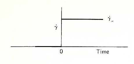
image: Middleman, S., Fundamentals of Polymer Processing, 1^st edition, McGraw-Hill, 1977. 

 The material equations previously given will now be modified to give the stress growth functions that can be used to describe the material.

Return to Main Page