PDF File: (Click to Down Load): Chapter3.pdf
Related Topic:
Semi-Crystalline Morphology in Polymers.html
Free Volume and Tg, WLF.html
Modulated DSC (Thermal Analysis Corp).html
Rheometers (Thermal Analysis Corp).html
Dynamic Mechanical Testing (Thermal Analysis Corp).html
Polymers typically display broad melting endotherms and glass transitions as major analytic features associated with their properties. Both the glass and melting transitions are strongly dependent on processing conditions and dispersion in structural and chemical properties of plastics. Characterization of polymers requires a detailed analysis of these characteristic thermal transitions using either differential scanning calorimeter (DSC) or differential thermal analysis (DTA). Additionally, polymers are viscoelastic materials with strong time and temperature dependencies to their mechanical properties. Temperature scans across the dynamic spectrum of mechanical absorptions are commonly required for characterization of polymers, especially for elastomers. These thermal/mechanical properties are characterized in dynamic mechanical/thermal analysis (DMTA). Additionally, weight loss with heating is a common phenomena for polymers due to degradation and loss of residual solvents and monomers. Weight loss on heating is studied using thermal gravimetric analysis (TGA).
A complete thermal analysis of a plastic sample yields inferential information concerning the chemical composition and structure of the material. Examples:
1. The Hoffman-Lauritzen description of the crystalline melting point associates shits in the melting transition temperature with the thickness of lamellar crystallites in polymers. Such structural based shifts would suggest further study using the Scherrer approach for diffraction peak broadening and small-angle x-ray and TEM analysis.
2. Dramatic weight loss in a TGA analysis of nylon at temperatures above 100deg.C indicate some association of water with the nylon chemical structure. Such an observation would suggest further study using spectroscopic techniques.
3. In a polymer alloy (blend), the observation of two glass transition temperatures indicates a biphasic system, a single glass transition, a miscible system following the Flory-Fox equation. Further support for miscibility would come from microscopy and scattering (neutron, x-ray and light can all be used to characterize miscibility).
Generally, thermal analysis is the easiest and most available of techniques to apply to a sample and for this reason thermal analysis is often the first technique used to analytically describe a plastic material.
Error analysis in thermal techniques usually is conducted by repetition of the measurement for at least 3 to 10 identical samples in order to determine the standard deviation in the measurement. In all thermal analysis techniques the instruments must be calibrated with standard samples displaying sharp and constant transition temperatures and enthalpies of transition.
Calorimetry (Differential Scanning Calorimetry, DSC; Differential Thermal Analysis, DTA):
Calorimetry involves the measurement of relative changes in temperature and heat or energy either under isothermal or adiabatic conditions. Chemical calorimetry where the heats of reaction are measured, usually involve isothermal conditions. Bomb or flame calorimeters involve adiabatic systems where the change in temperature can be translated, using the heat capacity of the system, into the enthalpy or energy content of a material such as in determination of the calorie content of food. In materials characterization calorimetry usually involves an adiabatic measurement. A calormetric measurement in materials science is carried out on a closed system where determination of the heat, Q, associated with a change in temperature, [Delta]T, yields the heat capacity of the material, C:
![]()
At constant pressure:
![]()
The enthalpy can be calculated from CP through,
![]()
Instrumentation for Thermal Analysis, DTA and DSC:
Figure 12.1 of Campbell and White shows a schematic of a differential thermal analysis (DTA) instrument. The instrument is composed of two identical cells in which the sample and a reference (often an empty pan) are placed. Both cells are heated with a constant heat flux, Q, using a single heater, and the temperatures of the two cells are measured as a function of time. If the sample undergoes a thermal transition such as melting or glass transition a difference in temperature is observed, [Delta]T = Tsample - Treference. Negative [Delta]T indicates an endotherm for a heating cycle. Quantitative analysis of DTA data is complicated and the instrument is usually viewed as a fairly crude sibling of a differential scanning calorimeter (DSC) discussed below. Recent instrumental advancements have improved the quantitative use of DTA instruments. A DTA instrument is generally less expensive than a DSC. Determination of transition temperatures are accurate in a DTA. Estimates of enthalpies of transition are generally not accurate. In the DTA heat is provided at a constant rate and temperature is a dependent parameter. In the equation above for CP, the normal order of dependent and independent parameters in the differential is reversed, so dT/dQ is actually measured rather than dQ/dT. This distinction is critically important in transitions where kinetics become important such as in polymer melting and glass transition.
Figure 12.2 of Campbell and White shows a schematic of a differential scanning calorimeter (DSC). The arrangement is similar to the DTA except that the sample and reference are provided with separate heaters. The independent parameter is the temperature which is ramped at a controlled rate. Feedback loops control the feed of heat to the sample and reference so the temperature program is closely followed. The raw data from a DSC is heat flux per time or power as a function of temperature at a fixed rate of change of temperature (typically 10Cdeg./min). Since the heat flux will increase with temperature ramp rate, higher heating rates lead to more sensitive thermal spectra. On the other hand, high heating rates lead to lower resolution of the temperature of transition and can have consequences for transitions which display kinetic features.
Campbell and White go through a useful 2 page comparison of the DSC and DTA techniques which should be reviewed.
Data Interpretation:
The output of a DSC is a plot of heat flux (rate) versus temperature at a specified temperature ramp rate. The heat flux can be converted to CP by dividing by the constant rate of temperature change. The output from a DTA is temperature difference ([Delta]T) between the reference and sample cells versus sample temperature at a specified heat flux. Qualitatively the two plots appear similar.
Both DSC's and DTA's must be calibrated, essentially, for each use since small changes in the sample cells (oil from fingers etc.) can significantly shift the instrumental calibration. For polymer samples these instruments are typically calibrated with low melting metal crystals that display a sharp melting transition such as indium (Tm = 155.8deg.C) and low molecular weight organic crystals such as naphthalene. The volatility of low molecular weight organic crystals requires the use of special sealed sample holders.
An instrumental time lag is always associated with scanning thermal analysis. The observed transitions may be "smeared" by this instrumental time lag (typically close to 1deg.C at 10deg./min heating rate). Some account can be made for this time lag by comparison of results from different heating rates. Often this time lag is accounted for by taking the onset of melting as the melting point rather than the peak value for sharp melting standard samples used in calibration. For polymer samples, significant broadening of the melting peak (up to 25 to 50Cdeg.) is the norm and this is associated with the structural and kinetic features of polymer melting. Typically the peak value is reported for polymer melting points. The instrumental error in temperature for a DSC is typically +/-0.5 to 1.0 Cdeg..
Typical DSC trace for a Semi-Crystalline Polymer:
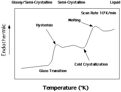
The Figure above is a typical schematic for a heating run on a quenched sample of semi-crystalline polymer such as polyethylene, polyester (such as PETE) or isotactic polystyrene (typical atactic polystyrene does not display a crystalline endotherm). The left axis is (dH/dT), Cp, or heat flux depending on the normalization of the heat flux. Also, the left axis is often plotted with the endotherm pointing down rather than up, flipping the curve. The curve can change dramatically with heating rate especially with respect to the hysteresis of the glass transition (residual enthalpy) and cold crystallization phenomena. The mechanical properties of the sample change from a brittle solid such as polystyrene at room temperature at the left, to a typical semi-crystalline material such as polyethylene in a milk jug in the middle to a viscous liquid like molasses to the right.
Determination of Tg:
To determine Tg two lines are drawn parallel to the baseline above and below the inflection at Tg. The midpoint of the departure from the left and the intersection with the baseline nearest Tg on the right is determined by the instrument. This midpoint is taken as the glass transition temperature. The residual enthalpy associated with Tg is sometimes also recorded from the high temperature baseline. This residual enthalpy will decrease with heating rate and has a strong dependence on the processing conditions of the sample and the length of time the sample is allowed to anneal near Tg. Tg is a second order transition since it displays a discontinuity in the derivative of the enthalpy (heat capacity). It is often termed a pseudo-second order transition because it displays a finite range of temperatures over which it occurs at finite heating rates and often displays a residual enthalpy.
Determination of Tm:
The melting point, Tm is determined, for broad melting polymers, by the temperature at the maximum in the (dH/dT) plot near this transition. The enthalpy of melting is determined by constructing a baseline above the melting and extending it to below any cold crystallization phenomena (exothermic peak below Tm and above Tg). Generally, the enthalpy of crystallization is taken as the area above this baseline. Sometimes the enthalpy of crystallization, which has occurred in the DSC measurement, is subtracted from this value to adjust the enthalpy as an estimate of the enthalpy associated with the original sample. The onset of melting is taken as the initial rise of the curve above baseline. The maximum melting temperature at this heating rate is taken as the final point which deviates from the baseline.
Melting Endotherm:
Gibbs-Thompson Relationship for Polymers (Hoffman-Lauritzen Theory): (Appendix 1)
In addition to the broad melting endotherms and the presence of cold crystallization as a dominant feature in semi-crystalline polymers a number of unique complications exist in the interpretation of calometric data. A variant of the Gibbs-Thompson equation, known as the Hoffman-Lauritzen equation governs the relationship between structure and melting point for lamellar crystallites which are present in essentially all semi-crystalline polymers. The Hoffman equation notes that there is a direct, inverse relationship between the undercooling at which the polymer crystallites melt and the thickness of the lamellar crystallites through:
![]()
where [Delta]T is the difference between the melting point of an infinite thickness and perfect crystallite and the observed melting point, [sigma]e is the free energy associated with the lamellar fold surfaces and dL is a term which accounts for the necessary deviation from equilibrium in the crystallization process. The latter term is usually neglected, i.e. dL ~ 0. The Hoffman approach gives rise to a possible description of the broad endotherm associated with melting of polymer crystallites, that is polydispersity in lamellar thickness. In many plastics, particularly in branched polyethylene, multiple melting endotherms are observed and the Hoffman relationship has been used to support the presence of discrete populations of crystallites associated, perhaps, with initial crystallization and formation of spherulitic structures, followed by decoration of spherulites by lower melting (i.e. thinner) lamellae.
A problem with the above analysis based on the Hoffman equation is that the degree of crystallinity (DOC) measured calorimetrically rarely agrees with that measured by XRD. XRD's DOC is usually taken as the best value since the myriad of complications which can be associated with a thermal measurement are mostly avoided. The value of the DOC obtained from thermal analysis, if all endotherms are included is usually higher than that of XRD which indicates that at least some of the endotherm measured calormetrically is associated with enthalpies of association present in the amorphous phase, such as tethered chains at the lamellar interface or interlamellar amorphous polymer. In some highly branched polyethylenes, it has been proposed that the bulk of the melting endotherm can be associated with such associated amorphous materials.
Melting Point Depression for Polymers: (Appendix 1)
The presence of miscible, non-crystallizing components are known to depress the melting point of all crystalline materials, i.e. adding salt to ice:
![]()
where a is the activity of the crystallizable component. Often the mole fraction of crystallizable component is substituted for the activity as an ideal approximation. In polymers, the non-crystallizable component can be a low-molecular weight impurity, but is often a non-crystallizable comonomer, an atactic segement, end-groups or a branch site. Substitution of the crystallizable fraction for "a" in the above equation yields the Sanchez-Eby Equation for copolymers. For low fractions non-crystallizable component, such as when considering end-group effects the log term can be approximated using, ln(a) ~ ln(Xcry) = ln(1-Xnoncry) ~ Xnoncry. For end-groups Xnoncry = 2M0/Mn, where M0 is the molecular weight of the end-group and Mn is the number average chain molecular weight. Thus, T0 for a polymer reflects the melting point of an infinite molecular weight sample.
For a thermodynamically miscible polymer or solvent at low concentrations the melting point depression can be expressed through a viral expansion where -ln(a) is replaced by a second order viral expansion involving the interaction parameter, [chi]:
![]()
where V represents molar volumes and [phi] is the volume fraction of solvent at low volume fractions. This equation is appropriate for melting point depression in the presence of a plasticizer for instance.
The melting point of a semi-crystalline plastic sample is strongly effected by distributions in morphology (lamellar thickness), impurity concentration and distribution in the sample, and processing history (thermal history) as well as the residual strain and orientation in the samples. All of these effects lead to a characteristically broad melting endotherm for plastics.
Glass Transition:
The melting point is a first order transition, in the Ehrenfest sense, since it involves a discontinuity in the first derivative of the Gibbs free energy with respect to temperature (-entropy) or pressure (volume). That is, there is a discontinuity in volume, for instance, at the melting point. The glass-transition, in the most ideal case, is a second order transition since the first derivatives of the Gibbs free energy are not discontinuous but the second derivatives with respect to temperature (-heat capacity/T), pressure (-volume * compressibility) and temperature/pressure (volume * thermal expansion) show a discontinuity. Polymers are unique in the dominance of the glass transition as the decisive factor in their mechanical properties. Polymers are the only material for which the equilibrium ground state is often glassy rather than crystalline. This is because topological and stereochemical constraints prevent the formation of crystals in many cases. The glass transition is often called a pseudo-second order transition because of the dominance of kinetics. Slower cooling rates in the DSC, for instance, lead to lower measured values of the glass transition. This time-temperature superposition is described by the Williams Landel Ferry (WLF) equation for example. This rate dependence hints at the basis of the glass transition in molecular motion. The glass transition is effected by orientation, rate, molecular weight, crosslink density and impurity content.
Molecular Weight (Flory-Fox Approach):
Through consideration of the free volume at the glass transition an expression can be obtained for the molecular weight dependence of the glass transition temperature which is based on the idea that chain ends lead to more free volume than mer units in the middle of chains:
![]()
where K is a constant (K = 2.1 x 10⁵ for polystyrene, with Tg,[infinity] = 106deg.C) and Mn is the number average molecular weight. The term K/Mn is proportional to the number of end groups as in the melting point equation above.
Polymer Blends (Fox Approach):
The Fox equation describes the glass transition temperature of a miscible blend of two polymers, a copolymer or a plasticized polymer:
![]()
where mi is the mass fraction of polymer "i". The Fox equation leads to a lower value of Tg than would be given by a simple linear rule of mixtures and reflects the effective higher free volume or randomness due to the presence of two components in a mixture.
Systems which obey the Fox equation are considered to display intimate and uniform mixing while those which deviate from it, especially those that display two glass transition temperatures are considered to be poorly mixed.
Tacticity and Tm/Tg:
Disubstituted vinyl polymers show dramatically different glass transition temperatures for different tactic forms (e.g. polymethylmethacrylate, PMMA: isotactic 43deg.C, atactic 105deg.C, syndiotactic 160deg.C). Monosubstituted vinyl polymers show a single glass transition temperature for the different tactic forms (e.g. polystyrene, PS, 105deg.C for all tactic forms). Melting points are generally dramatically different for different tactic forms since the different tacticities, i.e. isotactic versus syndiotactic, show different crystalline structures.
Thermal Gravimetric Analysis (TGA):
Many DTA instruments include the ability to measure mass as a function of temperature as well as the DTA output. In some cases such a thermal gravimetric analysis instrument is coupled with a mass spectrometer or an infrared absorption instrument for analysis of decomposition gasses. Typically, a superimposed plot of [Delta]Tsam-ref and weight can yield critical information concerning the changes which occur on processing a polymer. For instance, the thermal cycling of a processing operation can sometimes be mimicked in a DTA/TGA instrument to understand degradation and thermal transitions which effect the viscosity and other properties of a plastic. Often, a DTA/TGA analysis is used to define the processing limits for a polymer, at the lower temperature associated with the glass transition or melting point and at the upper temperature associated with degradation of the polymer. Polymers which absorb water, such as nylon, have been studied in depth using TGA instruments and an example of such a study is shown in figure 12.9 of Campbell and White.
Since the TGA instrument is fairly simple and self-explanatory it will not be extensively discussed.
Dynamic Mechanical Thermal Analysis (DMTA):
When a polymer is subjected to a forced mechanical vibration at a fixed frequency, temperature and elongation a fraction of the energy is absorbed and a fraction is returned elastically. This is evident if a rubber ball is dropped on the floor. The ball bounces back to a height, L', lower than the height from which it was dropped, L. The loss associated with the ball bouncing can be quantified as L" = L - L', for instance. If one were to vary temperature or speed of impact the rebound fraction would change. This will be demonstrated using a rubber ball cooled with liquid nitrogen in class.
In systems subjected to cyclic deformations or distortions, such as alternating current circuits, the loss term, L" is often associated with an imaginary component to a complex parameter, L*. So we would write, L* = L' + i L" where i is [radical](-1). In complex space, a 2-D plot with the x-axis real and the y-axis complex, the complex parameter L* is represented as a point and the angle, d, from the real or x-axis to a line from the origin to the point L* is given by: tand = L"/L'. tand is a "normalized" measure or the mechanical loss associated with the bouncing ball at a fixed temperature and frequency (speed of impact).
Any mechanical or rheological measurement can be conducted in a dynamic mode, i.e. with a sinusoidally oscillating force. For example, a tensile stress experiment involving an oscillating force, F([omega]) = F0 sin(2[pi][omega]t) where F0 is the amplitude of the force, [omega] is the frequency and t is the time in the inverse units of [omega], gives rise to a dynamic stress, [sigma]*([omega]) = F([omega])/A = [sigma]0 sin(2[pi][omega]t), where A is the sample's cross sectional area. The resulting strain, [epsilon]* = L([omega])/L0, for a viscoelastic material will display an in-phase component and an out of phase component, [epsilon]* = [epsilon]' sin(2[pi][omega]t) + [epsilon]" cos(2[pi][omega]t). More typically, the strain is the independent parameter, [epsilon]* = [epsilon]0 sin(2[pi][omega]t) and the stress is a complex response, since the material response is often a function of the maximum strain, [epsilon]0.
A complex Young's modulus can then be constructed, E* = E' + i E", with an associated reduced loss, E"/E' = tand. Similarly, a complex viscosity can be constructed for a shear experiment. Figure 12.10 in Campbell and White shows several arrangements for dynamic mechanical experiments.
Figure 12.11 in Campbell and White shows a typical measurement involving a glass and a crystalline transition for a semi-crystalline polymer. Below the glass transition the polymer is glassy and the elastic response is similar to a glass marble, i.e. E" is small and E' is large so tand = E"/E' is small. Above the glass transition the material is elastic and E" is small and E' is smaller. tand is slightly higher but lower than at Tg. At Tg, molecular motion leads to significant absorption at the frequency of the dynamic strain leading to a large E". E' is continuous through the transition so a peak in tand at the glass transition results. In class we showed that a rubber ball behaves like a piece of lead at the glass transition, i.e. a highly lossy material.
The real modulus, E', of the semicrystalline material in Figure 12.11 decays with temperature above the glass transition until the crystalline melting point where the material becomes a liquid. tand shows a monotonic increase until it peaks at the crystalline melting point due to enhanced molecular motion when crystals begin to melt.
In many polymers a number of absorption peaks are observed below the glass transition which can be associated with different types of molecular motion. The glass transition in this scheme is termed the primary transition temperature or a-transition, Ta, and the secondary transitions are labeled in sequence of decreasing temperature the [beta], [gamma], d and [epsilon] transitions with associated temperatures T[beta] for instance.
One of the uses for DMTA is in understanding the mechanical response of elastomers such as those used in tires. In a tire high frequency (low-temperature) loss is often considered good since it enhances the grip of a tire at high speeds (high frequency). Low frequency (high-temperature) loss is sometimes considered bad since it increases wear and reduces gas mileage. Elastomers can be tuned to broaden the mechanical absorption peak in certain temperature ranges by controlling chemical composition, chemical structure, and the structure of fillers such as carbon black which can make up more than half of the weight of a tire. The mechanical absorption spectrum is also critical to a wide range of plastics since the mechanical behavior of polymers varies with both temperature as well as speed of deformation through the time-temperature superposition principle.
Time-Temperature Superposition:
----Free Volume and Tg, WLF
In class a sample of silly-putty was used to demonstrate time-temperature superposition. If silly putty is left for a long period of time (minutes) it flows (liquid at long times, low frequency or high-temperatures). If a ball is made it will bounce (seconds, elastic at intermediate times, frequencies and temperatures). If silly putty is rapidly ripped apart it fails like a glass (glassy at very short times, high-frequency or low temperatures). From this observation we can consider that raising the temperature is similar to dropping the frequency or allowing more time for deformation.
Williams-Landel-Ferry (WLF) considered the equivalency of time and temperature in the context of free volume theory for an activated flow process in viscoelastic materials. The WLF equation yields an equivalent frequency for a given temperature relative to a ground state temperature and experimental frequency:
![]()
where C1 and C2 are constants for a given polymer and T0 is a reference temperature for a given polymer close to Tg. The constants in the WLF equation can be theoretically predicted from free-volume theory (C1 = 17.44 and C2 = 51.6, using T0 = Tg) or can be experimentally determined. Using the WLF equation a master curve can be constructed in temperature that corresponds to a standard frequency or a master curve in frequency can be constructed that corresponds to a standard temperature.
Ideal Models in the DMTA Measurement:
For an applied dynamic strain, [epsilon]* = [epsilon]0 sin(2[pi][omega]t), an ideal Hookean elastic will respond with a complex stress completely in phase with the applied strain:
[sigma]* = [sigma]0 sin(2[pi][omega]t) = E [epsilon]0 sin(2[pi][omega]t).
For a Hookean elastic E" = 0
For a Newtonian Fluid, an ideal viscous fluid, the stress is given by:
[sigma] = [eta](d[epsilon]/dt).
d[epsilon]/dt for the dynamic strain, [epsilon]* = [epsilon]0 sin(2[pi][omega]t), is given by:
d[epsilon]/dt = 2[pi][omega] [epsilon]0 cos(2[pi][omega]t),
so, for an ideal lossy material,
[sigma]* = 2[pi][omega] [epsilon]0 [eta] cos(2[pi][omega]t),
and E' = 0.
DMTA experiments can be performed on non-Newtonian fluids such as a polymer melt to determine the elastic component of a visco-elastic fluid or on a solid plastic or rubber to determine the viscous component of a visco-elastic solid.
Work of Dynamic Deformation:
The work performed in a DMTA measurement per unit sample volume per cycle, W, is given by:
![]()
The power consumed per unit volume is given by,
![]()
DMTA Measurement of Complex Shear Modulus:
One of the most common applications of DMTA measurements is the determination of the shear loss and storage modulus, G" and G' for a polymer melt. This measurement is critical to the understanding of polymer processing since a polymer melt is subjected to a variety of shear rates in a typical process. For example, in an extruder at early stages low shear melts polymer pellets and pressurizes the polymer fluid in the feed and melting zones of the extruder barrel. In the extruder die this pressurized melt is subjected to extremely high rates of shear as it is formed into the final extruded part. The energy consumed in the process is related to the complex shear modulus and the variation of the loss shear modulus with rate. For a dynamic shear strain,
[gamma]* = [gamma]0ei2[pi][omega]t = [gamma]0 sin(2[pi][omega]t)
where the shear strain is defined as the change in length of a fluid with respect to a normal direction. The complex shear stress, force per normal area dragging the fluid is given by Newton's viscosity law by,
![]()
The complex viscosity is written as,
![]()
(compare with complex modulus which is written E* = E' + iE"). The difference between this equation and that for the complex Young's Modulus occurs because the complex viscosity involves the measurement of the compliance of the fluid to an applied strain rate rather than the strain rate of a material due to an applied stress. The compliance, D, is the inverse of the modulus, E. For complex numbers the inverse is obtained by the ratio of the complex conjugate to the magnitude of the complex number:
![]()
The shear loss modulus, G", and shear storage modulus, G', are related to the dynamic viscosity [eta]* = [eta]' - i[eta]" by,
![]()
The Cox-Merz Rule gives the zero shear rate viscosity, [eta]0, as the magnitude of the complex viscosity,
![]()
2 Qualitative Examples of the Use of DMTA in the Plastics Industry:
1) In the processing of high density polyethylene a dramatic increase in the processing cost is associated with small amounts of long chain branching. This can be at levels below 5 branches per 1000 carbons in the main chain so can not be characterized using spectroscopic techniques. Rheological DMTA has been used to estimate the amount of long chain branching since the high-frequency shear loss modulus, G", displays a characteristic increase relative to the intermediate frequency loss modulus for branched materials. Presumably this effect is associated with hindrance of molecular motion at high frequencies due to the presence of long chain branches. There is good correlation between this measurement and the processing costs as well as some quantitative correlation between branch content and this mechanical response. DMTA is the only analytic technique which has been demonstrated to be sensitive to such weak chain branching and it has proven critical to control of synthesis conditions aimed at reduction of long chain branching in HDPE.
2) In the elastomer industry DMTA is a standard instrument for determination of the expected performance of rubber products. The most common example is a automotive tire which is subject to a wide range of dynamic strains in use. The frequency dependence of loss in elastomer compounds can be directly related to the performance of an elastomeric material in an automotive tire. The critical design criterion, in terms of materials, for a tire are "grip", "wear" and "fuel economy". The "grip" of a tire is usually associated with the high-frequency (low temperature) loss. The low-frequency (high temperature) loss is associated with the wear and loss of fuel economy. The addition of carbon black to an elastomer enhances the high frequency (low temperature) loss, leading to higher grip. The weight fraction of carbon in a tire is typically between 40 and 60%! In carbon reinforced elastomers, this higher grip is always associated with an increase in the low frequency response leading to an increase in energy absorption or reduced fuel economy for a tire as well as an associated increase in wear. The increase in loss with addition of carbon has been related to the association of elastomer molecules with filler, so called "bound-rubber content". Loss is also associated with breakup and re-formation of the loosely associated aggregates of carbon. In the design of elastomers for tire applications the goal is often to broaden the absorption peaks in the DMTA spectrum and to shift absorption's to higher frequencies through modification of the chemical structure of the elastomer and tuning of the filler structure.
Appendix 1: Gibbs-Thompson Equation and Melting Point Depression Equations
At the equilibrium melting point a crystal and its melt have equal Gibbs free energy, Gcrystal = Gmelt. For example, in a glass of water with ice cubes at close to 0deg.C the ice will fuse into a larger cluster due to epitaxial recrystallization (crystal surface nucleated crystallization). This occurs because there is little or no difference in free energy between water molecules in the liquid and crystalline states. An equilibrium melting point is defined as:
![]()
where [Delta] is the difference between the crystal and the melt and T[infinity] reflects ideal conditions.
There are many ways to deviate from this ideal situation. For example, the ideal crystal above is of infinite size. For real crystals, where surface area becomes important at small crystallite sizes the crystal will display an equilibrium with its melt at a different temperature due to the inclusion of a surface energy term:
![]()
A melting point depression is predicted for a finite sized crystal depending on the surface to volume ratio and the surface energy to bulk enthalpy ratio. For low surface energy crystals or for large crystals the effect is smaller. For polymers, crystallites are highly asymmetric with roughly the aspect ratio of a sheet of paper. This means that the A to V ratio is very large. Additionally, the planar surface of polymer crystals contain chain folds which have a high tortional energy associated with them. This means that the surface energy to enthalpy ratio is also large. Large under coolings are expected in polymer crystals and a direct relationship between the lamellar thickness and the melting point is predicted by the Gibbs Thompson Equation given above.
For a system such as a collection of red and blue marbles which are shaken up the entropy of the system can be calculated from combinatorial (or counting) statistics. The difference in entropy between a segregated state (all blue at the top and all red at the bottom) and a totally mixed state (blue and red randomly dispersed) is given by the total number of ways to arrange the marbles in the dispersed state, [Omega]:
![]()
If an impurity is added to a crystal and it has a totally uniform dispersion then a change in entropy between the pure crystal and the crystal with the dispersant can be calculated form a combinatorial approach which parallels the red and blue marble law above assuming that the number of states increases with the molar concentration of the impurity, x:
![]()
Using an approach similar to the Gibbs Thompson discussion above, a melting point depression can be predicted:
![]()
rearranging:
![]()