PDF File: (Click to Down Load):
Chapter2.pdf
=> Back to TOC
=> To Syllabus
Parts:
=> Equation of Continuity
=> Vectors and Tensors
=> Tensors in Flow
=> Newtonian Fluids
=> Lubrication Approximation
=> Reynold's Equation
=> Normal Stresses
Chapter 2, Transport Phenomena
Tadmor Chapter 5
Chapter 5 of Tadmor is an overview of rheology that basically summarizes the first few chapters of "Transport Phenomena" by Bird, Stewart, Lightfoot which is the standard Chemical Engineering text on this subject. The development begins with a discussion of equations of continuity in simple terms, then reviews vectors and tensors and applies these to continuity in flow. Application of typical assumptions in vector form and development of the Reynold's Equation follow. A brief discussion of the Lubrication Approximation is given in the context of the Reynold's Equation.
Balance Equation
(Equation of Continuity)
Kinetic processes, i.e. a process that is characterized by rates and non-equilibrium (non-thermodynamic) features, are described by equations based on the simplist laws of the world as we know it, laws of conservation of mass, energy and momentum. The principle of conservation simply states that
1) if one constructs a box around a part of the universe,
2) then one can consider that within the box the total amount of mass, for instance, is conserved, i.e. mass is not created out of nothing in normal life (this does not necessarily apply to the begining of the universe for instance). Mass can be formed, but in some predictable way governed by equations that may be empirical or fundamental.
The use of such equations of continuity, then, require you to consider the part of the universe you are interested in, and to construct a closed set of borders around which you will perform a mathematical balance of mass, energy or momentum. The construction of the box is the crucial step in this process since the mathematics is simply a form of bookkeeping.
Consider, for instance, the population of Cincinnati. Of the many possible results for this question all require that you define, at the first step 1) what it is that you mean by "Cincinnati"; 2) what it is that you mean by "population". The usefullness of the result is strongly dependent on your formulation of the question. If population is defined as number of living people at a given time on a scale of seconds then it will be necessary to determine the rate of traffic on all interstates in and out of the city, the rate of air traffic, birth rates, death rates. Some estimate of the total population at a given instant of time would be necessary. Additionally, a border needs to be defined that could include only downtown or could include the I-275 boundary, or regions with population density more than 2,000 per square mile for instance (the box). If the population were defined as voting age adults, a much more complicated algorithm would be necessary and political boundaries would probably be appropriate. From this example it should be clear that the problems associated with equations of continuity mainly involve your view of the problem including definition of terms and construction of a box. The math involved in summing rates is fairly trivial although it can appear imposing when tensoral forms are included.
Features of Continuity Equations (CE's):
- CE's can be written for energy, mass, or momentum. They assume either energy, mass or momentum are conserved and are thus based on the basic principles of physics. Each of these three types can be specified further, e.g. the mass of water in a boiling pot, the momentum of planets in the solar system (doesn't include space ships for instance).
- CE's use constitutive equations and constitutive constants as well as basic laws of physics to account for loss and gain.
- CE's become mathematically complicated since transport can occur in 3-d space, i.e. CE's naturally involve vectors and tensors.
- The concept of a CE is very simple, it involves a black box approach to a process,
IN = OUT + CHANGE
e.g. for mass in a continuous process (flow process),
Rate of Mass In = Rate of Mass Out + (Rate of Change of Mass)
- The last term is 0 for steady state.
- Consider a box with flow only on two sides, vy = vz = 0 :
Rate of Mass In - Rate of Mass Out = Rate of Change in mass
-d(rvx)/ dx = dr/ dt
Takeing a partial derivative on the left and rearranging:
dr
/ dt + vx dr/ dx = - r dvx/ dx
d
vx/ dx is the elongational strain rate (remember dg/dt = dvx/ dy)
- Even for the simple scenario of #6 the definition of
dg/dt is not sufficient, i.e. for vx we have at least 3 components: dvx/ dx, dvx/ dy, dvx/ dz .
There are 9 components to the velocity gradient tensor if vx, vy and vz have values.
- Often the diagonal components of this 9 component tensor are zero, i.e. there is no elongation associated with steady state.
- Similarly, the simple definition of the shear stress,
t
xy = dFx/dAy
is insufficient. The tensile stress is txx for instance.
The total stress tensor p, has 9 components
- The diagonal components of the total stress tensor are the tensile stress components. For an incompressible fluid (usually assumed) the sum of the diagonal components is 0 (constant hydrostatic pressure).
- The main point is that it is necessary to talk of the tensoral nature of stress and strain even in the simplest situations. This becomes even more important for non-Newtonian fluids.
Review of Vector and Tensor Math Operations.
- The dot product of two vectors is given by:
v . w = vw cosfvw (a scalar)
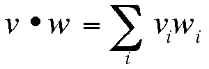
The dot product is a projection of one vector on another times the second vector's magnitude.
- The cross product of two vectors is given by:
v x w = nvwvw sinfvw (a vector)
nvw is a vector normal to the vw plane and has magnitude of 1
v x w = d1 d2 d3
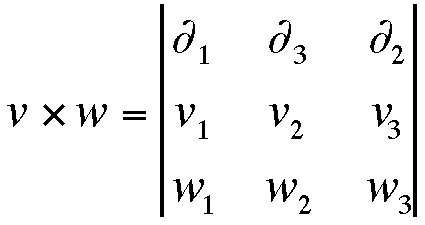
The cross product is the area created by two vectors and has the direction of the normal to the plane created by the two vectors using the right-hand rule.
- The del-operator is given by
—
= d1 (d/dx1) + d2 (d/dx2) + d3 (d/dx3)
where di are unit operators, and
d1 = 1 for i=1 and = 0 for i not equal to 1.
- The substantial derivative is given by:
D/Dt = d/dt + v . —
- The gradient of a scalar is a vector:
— (scalar).
- The divergence of a vector is a scalar: —.(v) or div(v).
- The curl of a vector is a vector:
—x(v) or curl(v).
- The Diadic Product of a vector is a tensor:
—v or curl(v).
Equation of Continuity Using Tensor Math
The simple equation of continuity for unidirectional flow,
dr/ dt = - d/dx1(r v1) can be easily converted to tensor form,
dr/ dt = -(— . r v)
Similarly, the short hand form for: dr
/ dt + v1 dr/dx1 = -r dv1/dx1, is given by:
Dr/Dt = - r(— . v) (= 0 for incompressible fluid)
Velocity Gradient Tensor, —v
(pp. 115 in Tadmor)
The velocity gradient tensor is given by:
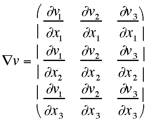
—
v contains two easily distinguishable tensoral components
- The rate of strain tensor:
dg/dt = —v + —vt
where —vt is the transpose of the velocity gradient tensor
dg/d
t gives rise to the net directional flow in a process. This is the useful flow.
- The vorticity tensor:
—w = —v - —vt
w gives rise to rotational flow which wastes energy but gives no net flow.
We are usually interested in the Net flow so dg/dt is of primary interest.
The velocity gradient tensor is defined in terms of the rate of strain tensor and the vorticity tensor by:
—v = 1/2(dg/dt + w)
Total Stress Tensor, p
(pp. 110 in Tadmor)
The total stress tensor is given by,
Some features of the total stress tensor are given below:
- pij = pji
i.e. the matrix is symmetric so the tensor has only 6 unique components.
- The total stress tensor can be broken down into two natural components.
- Hydrostatic pressure, d P
P 0 0
0 P 0
0 0 P
The hydrostatic pressure is an isotropic matrix not associated with net> flow.
- Shear Stress Tensor t,
t = p - Pd
The shear stress tensor is a symmetric tensor associated with net flow.
- The total stress tensor is given by:
p = Pd + t
Tensor Invariants
The components of a tensor matrix, such as the total stress tensor, change with the choice of coordinate system. That is if Cartesian coordinates are used for pipe flow, different tensor matrix components will result than if cylindrical coordinates are used. Additionally, if the reference frame even using Cartesian coordinates is rotated then the matrix will completely change. If the tensor itself does not change then there are some features of the tensor that can be calculated from any coordinate system that remain unchanged on change of coordinate system. These features are called the tensor invariants.
Several features of invariants are given below:
- Vectors have one derived value which doesn't change with coordinate system, the magnitude. 3x3 Tensors have 3 invariants , i.e. derived values which do not change with coordinate system.
- Invariants are scalars that are intimately related to a vector or tensor.
- While the constituent values of a 3x3 tensor changes with coordinate system. There are some derived values which are coordinate system invariant , i.e. the hydrostatic pressure for example. The three invariants for a 3x3 tensor can be defined in several ways. One accepted way is:
- I = Si tii
- II = Si Sj tijtji alternatively written II = t:t
- III =
Si Sj Sk tijtjktki
- The shear rate is (IIdg/dt)1/2/2 = 1/2 {(dg/dt) : (dg/dt)}1/2
Newtonian Fluid
(Constitutive Equation)
For a fluid with a viscosity that does not change with shear rate we can write as a constitutive equation:
t
= h dg/dt - (2/3 h - k) (—.v) d
where k is the dilatational viscosity. For an incompressible fluid, (—.v) = 0 .
The Navier-Stokes Equation is the equation of continuity for Newtonian fluids of constant viscosity and constant density,
r
Dv/Dt = -—P + h —2v + rg
where —2 is —.—
For creeping flows (polymers) viscosity dominates over inertia (
—2v) and the Navier-Stokes equation becomes:
r dv/dt = -—P + —. t+ rg
Common Assumptions
In solving the Navier-Stokes equation for a given rheological system several common limiting conditions and assumptions are made:
- No Slip at Wall: The fluid next to a wall moves at the same velocity as the wall.
- Liquid/Liquid Interface
- No Slip
- Continuous Stress
- Normal stresses and surface forces balance through interface curvature.
- Steady State: No change in response with time, In=Out, in general:
d/dt = 0
- Constant Properties in T & P
Heat conductivity, K
Heat Capacity Cp
Density r
1) You will know if this fails=> Melt Fracture, Stick-slip (eraser behavior)
2) P1 - P0 = g (1/Rx - 1/Ry) Pressure difference is related to two dimensions of surface curvature.
Lubrication Approximation
(Reynolds Equation)
A low viscosity fluid in a thin gap is equivalent to a high viscosity fluid in a wide gap since the Reynolds number, Re, is the same,
Re = R r V/h
where R is the gap size, r is the density, V is the velocity.
If Re is bigger than 2000 the flow becomes turbulent
For two systems with the same Reynolds number the flow is said to be similar, i.e. a polymer melt in and extruder is like a lubricating oil in a narrow gap.
Some assumptions on which the Lubrication Approximation (Reynolds Equation) is based are given below:
- Laminar Flow:
- This is flow which is like shearing a deck of cards.
- Flow is in one direction only , x.
- Flow is a continuous function of y (i.e. no discontinuities, i.e. no slip)
- Steady State
- In = Out
- Isothermal: Heat in = heat out
- Incompressible: Mass in=Mass out
- Newtonian (Viscosity is constant in
dg/dt):
t = h dg/dt .
(For non-Newtonian h = f(dg/dt) .)
Viscosity dominates over inertia (Creeping Flow), i.e. a couette viscometer is flow of two flat plates.
Taking Navier-Stokes, r Dv/Dt = -—P + h —2v + rg, for these conditions,
—
P = h —2v and for velocity only in the x direction,
dP/dx = h d2vx/dy2
which on integration yields:
vx(y) = Vx(1 - y/H) + H/2h (dP/dx) y(y/H -1)
where v = Vx at y = 0 and v = 0 at y = H. The pressure driven velocity is maximum in the middle. The first term in this form of the Reynolds Equation is linear and the second is parabolic. The sum gives a skewed parabolic profile.
For Reynolds flow between 2 plates, integration over y yields:
qx = VxH/2 +H3/12h (-dP/dx)
Details of Reynold's Equation.html
Details of Reynold's Equation.pdf
Hydrostatic Pressure and Normal Stresses
As discussed in chapter 1, polymers subject to shear will develop pressures normal to the direction of flow. These forces are termed normal forces. Normal forces act in the same direction as the components of hydrostatic pressure discussed in this section. Then it is important draw a distinction between hydrostatic pressure and normal forces in the sense that they are considered in polymer flow. This is natural to do in the framework of the total stress tensor, hydrostatic pressure and shear stress tensor discussed above. The total stress tensor is given by:
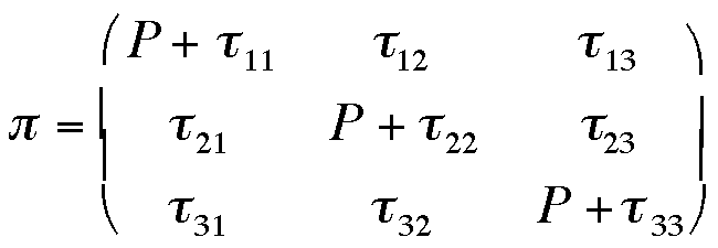
where the hydrostatic pressure is represented by P.
Since each of the diagonal components contains the hydrostatic pressure it is not possible to independently measure the normal stress. One can only consider differences between the 3 diagonal components of the matrix, defining two independent normal stres differences:
1'st normal stress difference = Y1 = t11- t22 = p11- p22
2'nd normal stress difference = Y2 = t22- t33 = p22- p33
(Shear stress = t12)
PDF File: (Click to Down Load):
Chapter2.pdf
=> Back to TOC
=> To Syllabus